A newer version of this visualization is available.
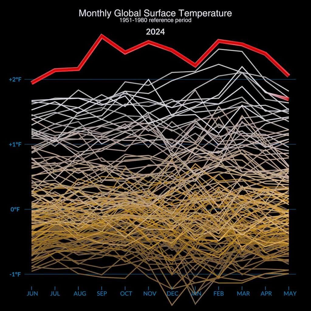
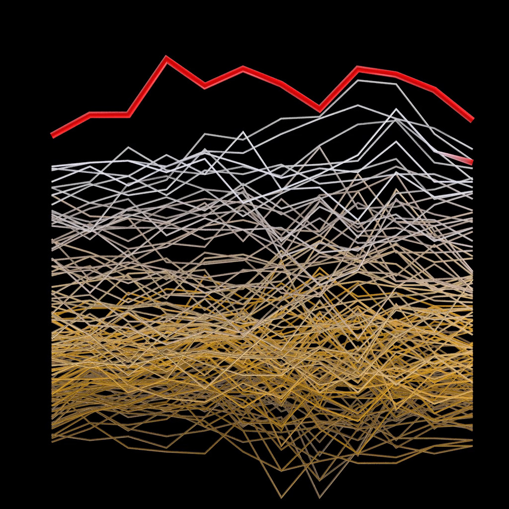
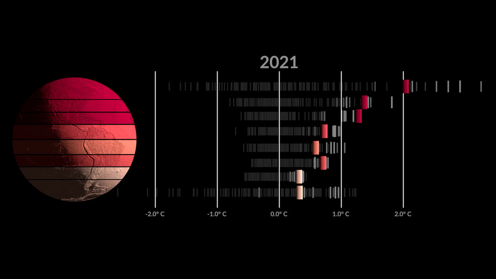
Shifting Distribution of Land Temperature Anomalies, 1962-2022
The change in the distribution of land temperature anomalies over the years 1962 to 2022. This version is in Celsius, a Fahrenheit version is also available.
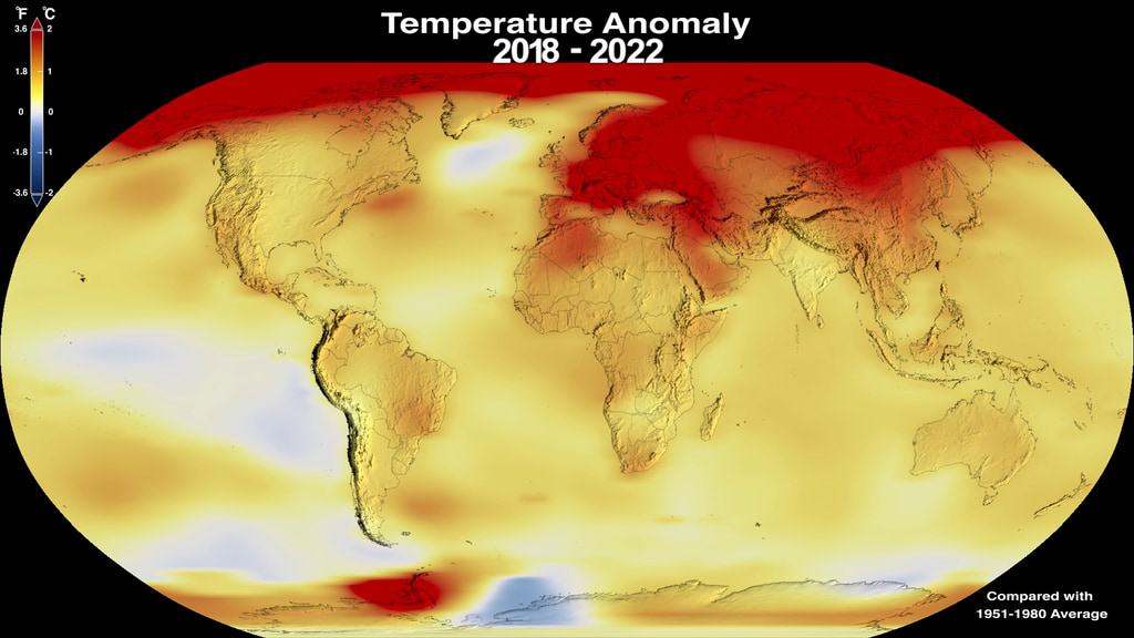
What we’re seeing: A temperature anomaly is a way of measuring how far air or water temperatures have strayed from a baseline average. Showing how much Earth’s temperature has warmed or cooled compared to a norm is an important way of visualizing how our climate is changing.
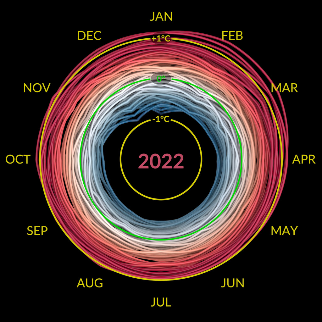
The data visualization above shows how air temperatures between 1962 and 2022 departed from the average for 1951-1980. (The anomalies have been plotted in degrees Celsius; a Fahrenheit version of the same animation is available in the plot below.) The darker shades of blue represent times when temperatures were significantly cooler than the norm and the orange and red represent times when temperature was hotter than the norm.
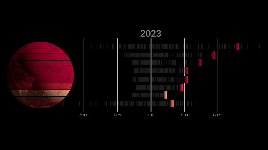
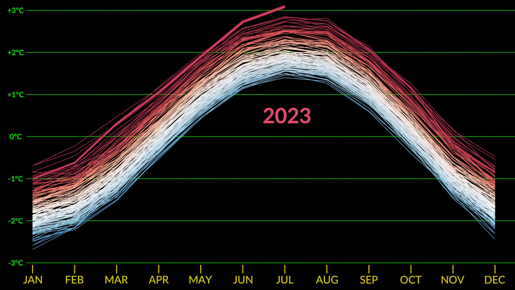
Why does the distribution wobble and change shape?: In this graph, 0 on the x-axis represents that average baseline. As the years tick by, you can see the average annual temperature shift in relation to that line. The y-axis shows the frequency of occurrence, meaning how often the annual temperature was at, above, or below the baseline.
Over time, the distribution progressively shifts to the right and broadens: This indicates that global air temperature is persistently warming. The shortening and widening of the distribution represents a wider range of temperature extremes. Once the animation reaches 2022 – tied for the fifth warmest year on record – the peak is roughly at 1.2 degrees Celsius (2.1 degrees Fahrenheit) warmer than the baseline.
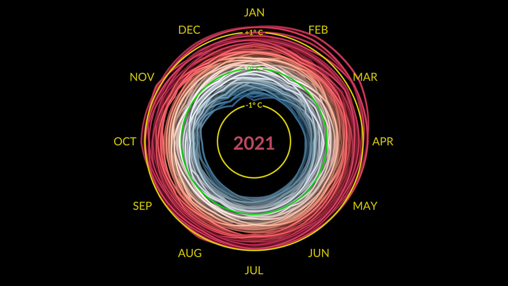
El Niño, La Nina, and ‘the Climate Jellyfish’: The bobbing back and forth of the curve shows the influence of El Niño and La Nina. El Niño is a natural climate phenomenon characterized by warmer than normal sea surface temperatures (and higher sea levels) in the central and eastern tropical Pacific Ocean. The planet is typically warmer in the El Niño phase and cooler in the La Nina phase. For context, 2020-2022 were all La Nina years, while 2015-16 were El Niño years.
Because of the nature of this movement, Mark SubbaRao, who leads NASA’s Scientific Visualization Studio and created the animation, gave it the nickname, “the climate jellyfish.”
“It looks like a jellyfish, right?” he said. “The jiggling back and forth, bobbing and weaving, there’s an organic nature to it.”
Where the data comes from: This visualization uses data from the NASA’s Goddard Institute of Space Studies (GISS) surface temperature analysis, known as GISTEMP. This analysis is based on calculating temperature anomalies rather than absolute temperature.
GISTEMP relies on millions of observations from thousands of weather stations, Antarctic research stations, ships, and ocean buoys. NASA’s full surface temperature dataset – and the complete methodology used to make the temperature calculation – is available here.
GISS is a NASA laboratory managed by the Earth Sciences Division of the agency’s Goddard Space Flight Center in Greenbelt, Maryland. GISS is affiliated with Columbia University.
Why measure temperature anomalies rather than absolute temperatures?: Absolute temperature can vary enormously over short distances — think a valley and a nearby mountaintop — but temperature anomalies stay largely consistent over bigger regions. If it’s above average for the month in Washington, DC, it will likely also be above average in Philadelphia, New York City, and Richmond, Virginia.
Also some areas — the Sahara Desert or the Arctic, for example — have fewer ground stations for measuring temperature. Because stations are not uniformly distributed, scientists rely on anomalies to more accurately account for areas lacking direct observations.
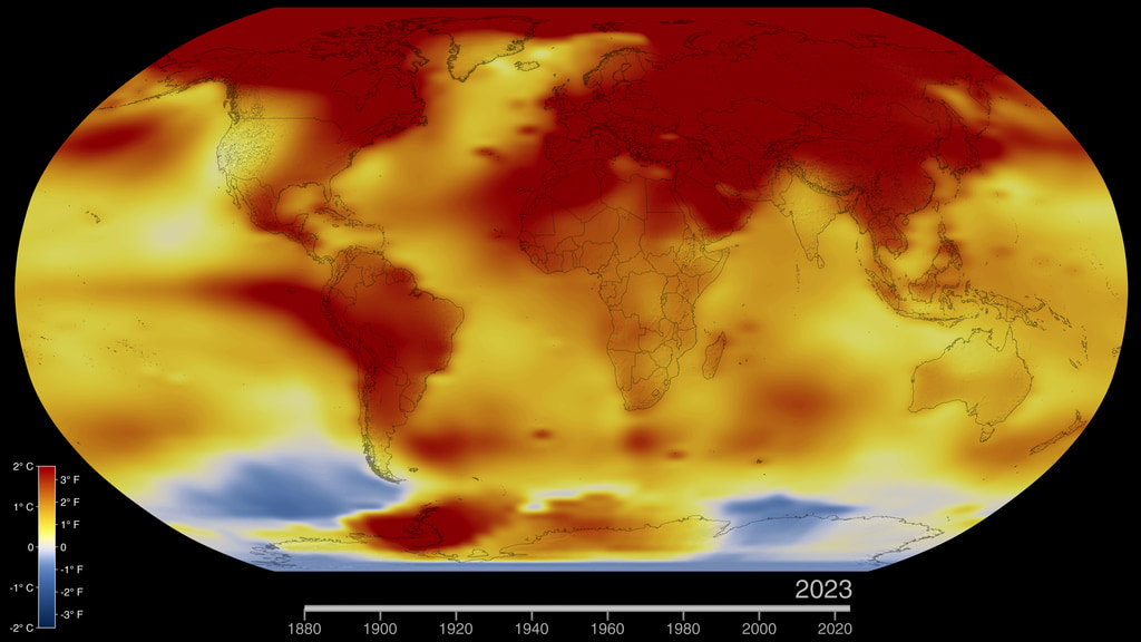
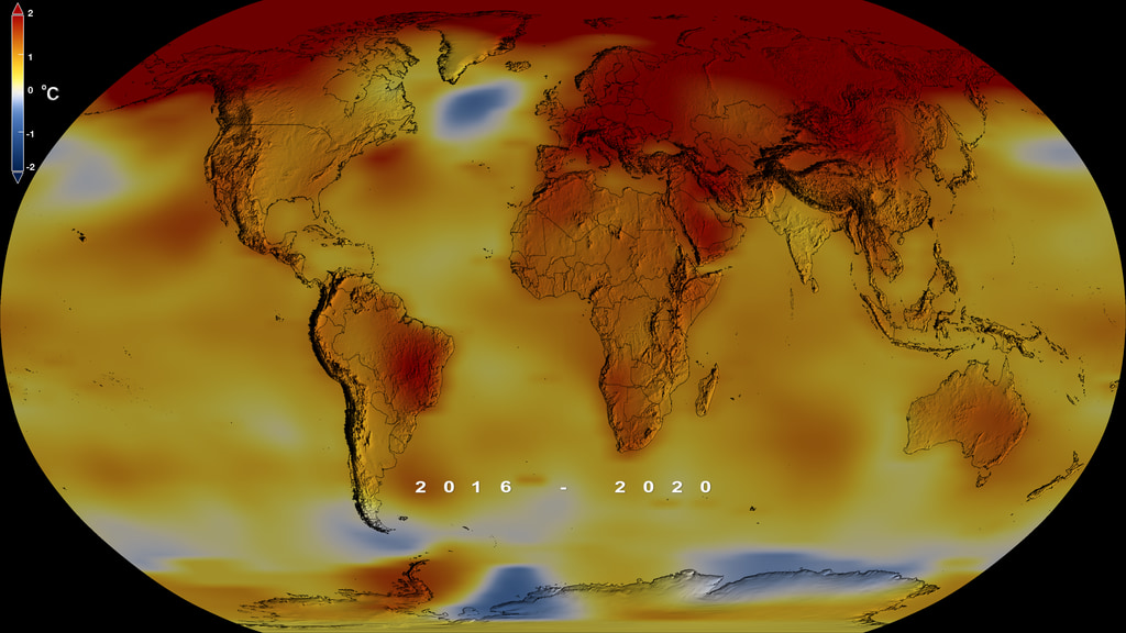
Why it matters: The visualization reflects a long trend of warming. We know from a tremendous amount of evidence that human activities are driving this trend.
By the year 2022, you can see two things happening in this visualization. The average temperature on Earth has increased, and extreme temperatures – especially extreme heat – have become more common.
“What this graph shows you is the magnification effect of warming combined with the broadening temperature distribution,” SubbaRao said. “It is more than just shifting everything by 1.2 degree Celsius. The broadening leads to more extreme temperatures as well. The climate is changing, and graphs like this give you insight into how it’s changing.”
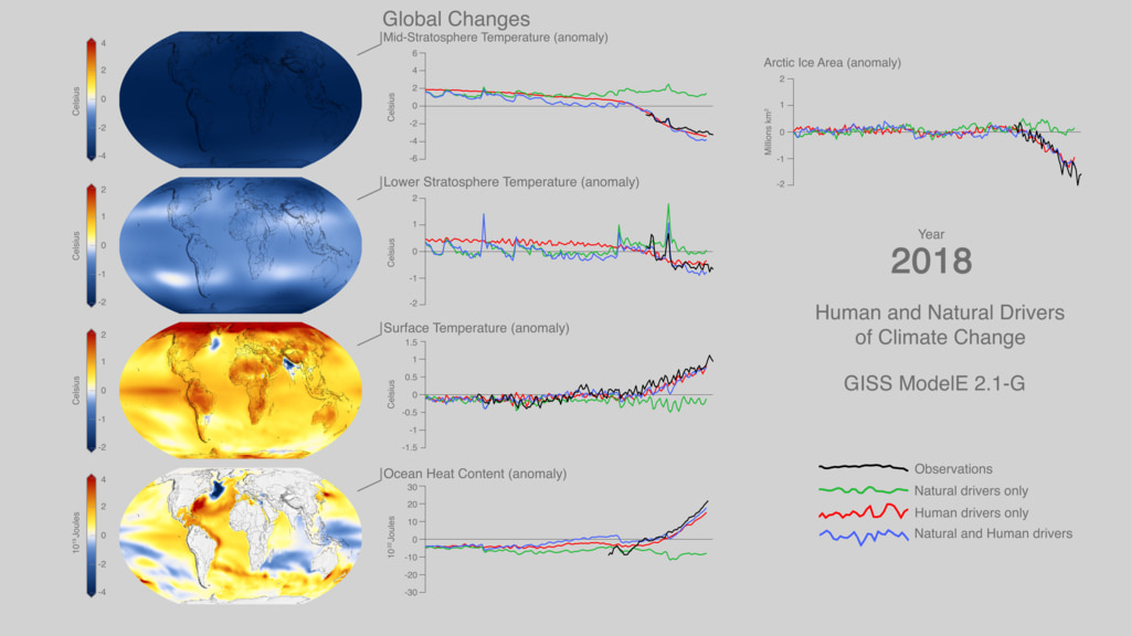
To understand how and why our planet is changing this way, NASA monitors temperatures, volcanoes, the Sun, and greenhouse gases, said Gavin Schmidt, NASA climate scientist and the director of GISS.
“It involves piecing together all the different fingerprints we are seeing, from the stratosphere to the surface to the ocean and from the tropics to the poles,” Schmidt said. “Unfortunately, when you put all of that together, what you find is that the trends that are driving these record temperatures and record heat waves are due to our activities. And it’s the emissions of greenhouse gases that are the dominant theme in all of that.”
“That’s not great to hear,” he added, “but that is what the science says.”
Explore this dataset: NASA’s full surface temperature data set – and the complete methodology used to make the temperature calculation – are available at: https://data.giss.nasa.gov/gistemp. A python based Jupyter Notebook which access the data and creates these visualizations is available. Click here to download.
The change in the distribution of land temperature anomalies over the years 1962 to 2022. This version is in Fahrenheit, a Celsius version is also available.
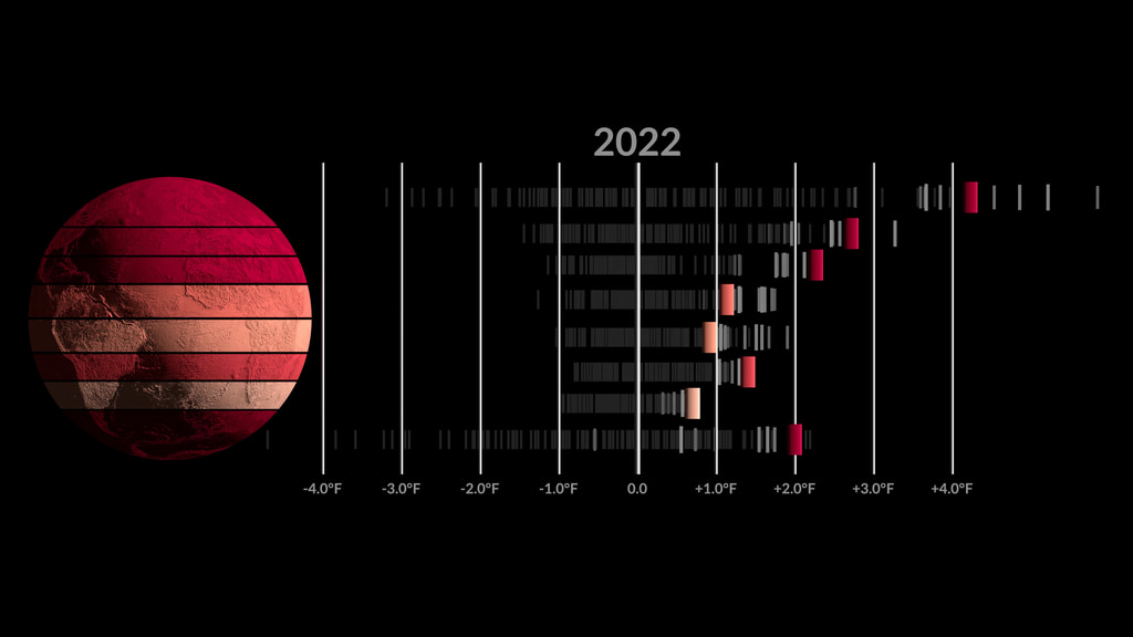
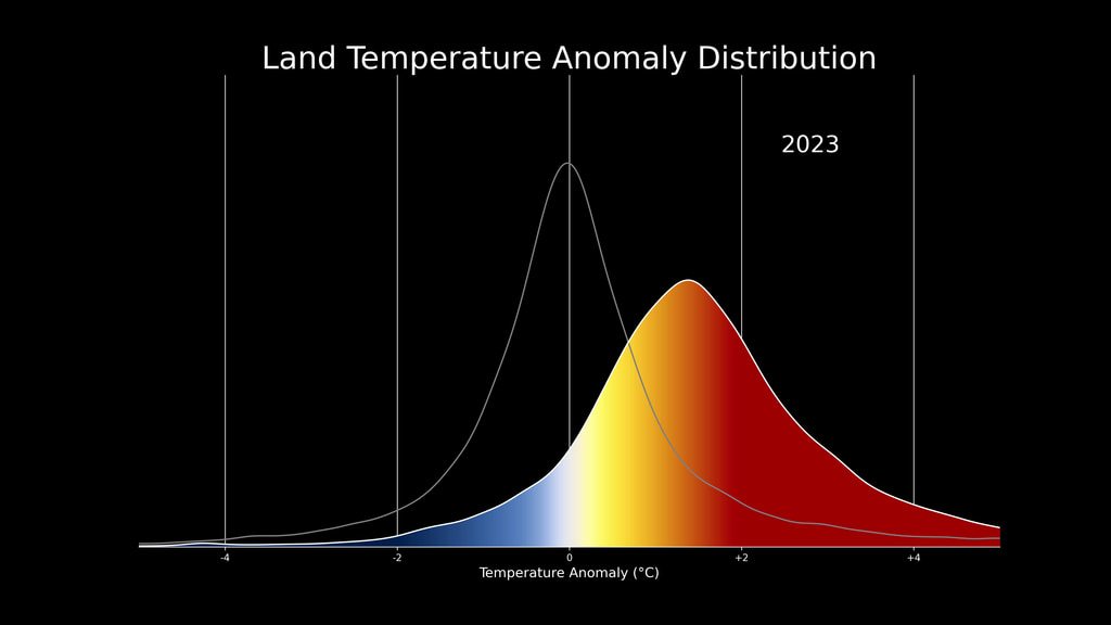
Descriptive Text for the Visualization: The visualizations start with a graph showing the global distribution of temperature anomalies. At the top of the graph is a title that reads ‘Land Temperature Anomaly Distribution’ and at the bottom is the x-axis label that reads ‘Temperature Anomaly’. The distribution is bell shaped, with a peak just slightly left of the center zero-degree mark, rising nearly to the top of the graph. The width of the bell-shaped distribution is approximately one degree Celsius (1.8 degrees Fahrenheit). The area under the curve is colored with the area to the left of the center zero line progressively darker and darker shades of blue and the area to the right of center progressively darker and darker shades of red representing warmer temperatures. In the upper right a label indicates indicates the year, starting at 1962.
As the visualization plays the year runs from 1962 to 2022, and the distribution wobbles back and forth and bobs up and down. The motion has led to this visualization being nicknamed ‘the climate jellyfish’. On top of this wobbling, as the visualization progresses the distribution progressively shifts to the right and broadens. Every 20 years a grey trace of the distribution is left behind, illustrating the change over time. Once the animation reaches 2022 the peak is roughly at 1.2 degrees Celsius (2.1 degrees Fahrenheit), and the distribution has broadened so that it is now almost twice as wide as it was in 1962 and roughly two-thirds as high. The visualizations end showing the distributions of 1962, 1982, 2002, and 2022 illustrating the evolution of the temperature distribution over time.
Credits
Please give credit for this item to:
NASA's Scientific Visualization Studio
-
Visualizer
- Mark SubbaRao (NASA/GSFC)
-
Technical support
- Laurence Schuler (ADNET Systems, Inc.)
- Ian Jones (ADNET Systems, Inc.)
-
Scientists
- Gavin A. Schmidt (NASA/GSFC GISS)
- Helga (Kikki) Kleiven (University of Bergen)
-
Advisor
- Peter H. Jacobs (NASA/GSFC)
-
Web administrator
- Ella Kaplan (Global Science and Technology, Inc.)
-
Writer
- Jenny Marder Fadoul (Telophase)
Release date
This page was originally published on Wednesday, May 31, 2023.
This page was last updated on Monday, May 29, 2023 at 11:23 PM EDT.
Datasets used in this visualization
-
GISTEMP [GISS Surface Temperature Analysis (GISTEMP)]
ID: 585The GISS Surface Temperature Analysis version 4 (GISTEMP v4) is an estimate of global surface temperature change. Graphs and tables are updated around the middle of every month using current data files from NOAA GHCN v4 (meteorological stations) and ERSST v5 (ocean areas), combined as described in our publications Hansen et al. (2010) and Lenssen et al. (2019).
Credit: Lenssen, N., G. Schmidt, J. Hansen, M. Menne, A. Persin, R. Ruedy, and D. Zyss, 2019: Improvements in the GISTEMP uncertainty model. J. Geophys. Res. Atmos., 124, no. 12, 6307-6326, doi:10.1029/2018JD029522.
This dataset can be found at: https://data.giss.nasa.gov/gistemp/
See all pages that use this dataset
Note: While we identify the data sets used in these visualizations, we do not store any further details, nor the data sets themselves on our site.
Related
- ID: 5311
- ID: 5327
- ID: 5207
 Visualization
 - ID: 5209
 Visualization
 - ID: 14502
 Produced Video
 - ID: 5191
 Visualization
 - ID: 5190
 Visualization
 - ID: 5161
 Visualization
 - ID: 5137
 Visualization
 - ID: 5057
 Visualization
 - ID: 5059
 Visualization
 - ID: 5060
 Visualization
 - ID: 4978
 Visualization
 - ID: 4975
 Visualization
 - ID: 4964
 Visualization
 - ID: 4908
 Visualization
 - ID: 4882
 Visualization
Newer Versions
- ID: 5211
Older Versions
- ID: 3975
Used as a Source In
- ID: 13979
![Music: Futurity by Lee Groves [PRS] and Peter George Marett [PRS]Complete transcript available.](/vis/a010000/a013900/a013979/Screen_Shot_2021-10-28_at_2.29.18_PM.png)