SDO: 4k Content
Overview
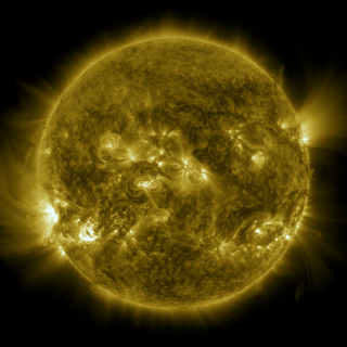
Since 2010, the Solar Dynamics Observatory has taken 60 million images of the sun and 2 comets. Here are a few of our favorites.
2024
- ID: 5216
 Visualization
 - ID: 5215
- ID: 14531
 Produced Video
 - ID: 5225
 Visualization
 - ID: 5224
 Visualization
 - ID: 5223
 Visualization
 - ID: 5220
 Visualization
 - ID: 5218
 Visualization
 - ID: 5239
 Visualization
 - ID: 5233
 Visualization
 - ID: 5232
 Visualization
 - ID: 5231
 Visualization
 - ID: 5244
 Visualization
 - ID: 5243
 Visualization
 - ID: 5246
 Visualization
 - ID: 5245
- ID: 5268
 Visualization
 - ID: 5256
 Visualization
 - ID: 5255

- ID: 14592
 Produced Video
2023
- ID: 5210
 Visualization
 - ID: 5206
- ID: 5205
- ID: 5203
 Visualization
 - ID: 5204
 Visualization
 - ID: 5202
 Visualization
 - ID: 5201
 Visualization
 - ID: 5167
 Visualization
 - ID: 5166
 Visualization
 - ID: 5140
 Visualization
 - ID: 5139
 Visualization
 - ID: 5138
 Visualization
 - ID: 5128
 Visualization
 - ID: 5125
 Visualization
 - ID: 5108
 Visualization
 - ID: 5103
 Visualization
 - ID: 5096
 Visualization
 - ID: 5085
 Visualization
 - ID: 5084
- ID: 5083
 Visualization
 - ID: 5080
 Visualization
 - ID: 5079
 Visualization
 - ID: 5082
- ID: 5077
 Visualization
 - ID: 5063
- ID: 5066
 Visualization
 - ID: 5068
 Visualization
 - ID: 5062
- ID: 5055
- ID: 5109
2022
- ID: 5016
 Visualization
 - ID: 5102
 Visualization
 - ID: 5042
 Visualization
 - ID: 14202
 Produced Video
 - ID: 14163
 Produced Video
 - ID: 5008
 Visualization
 - ID: 14160
 Produced Video
 - ID: 5005
 Visualization
 - ID: 5000
 Visualization
 - ID: 4999
 Visualization
 - ID: 5015
 Visualization
 - ID: 4998
- ID: 4966
 Visualization
2021
- ID: 13982 Produced Video

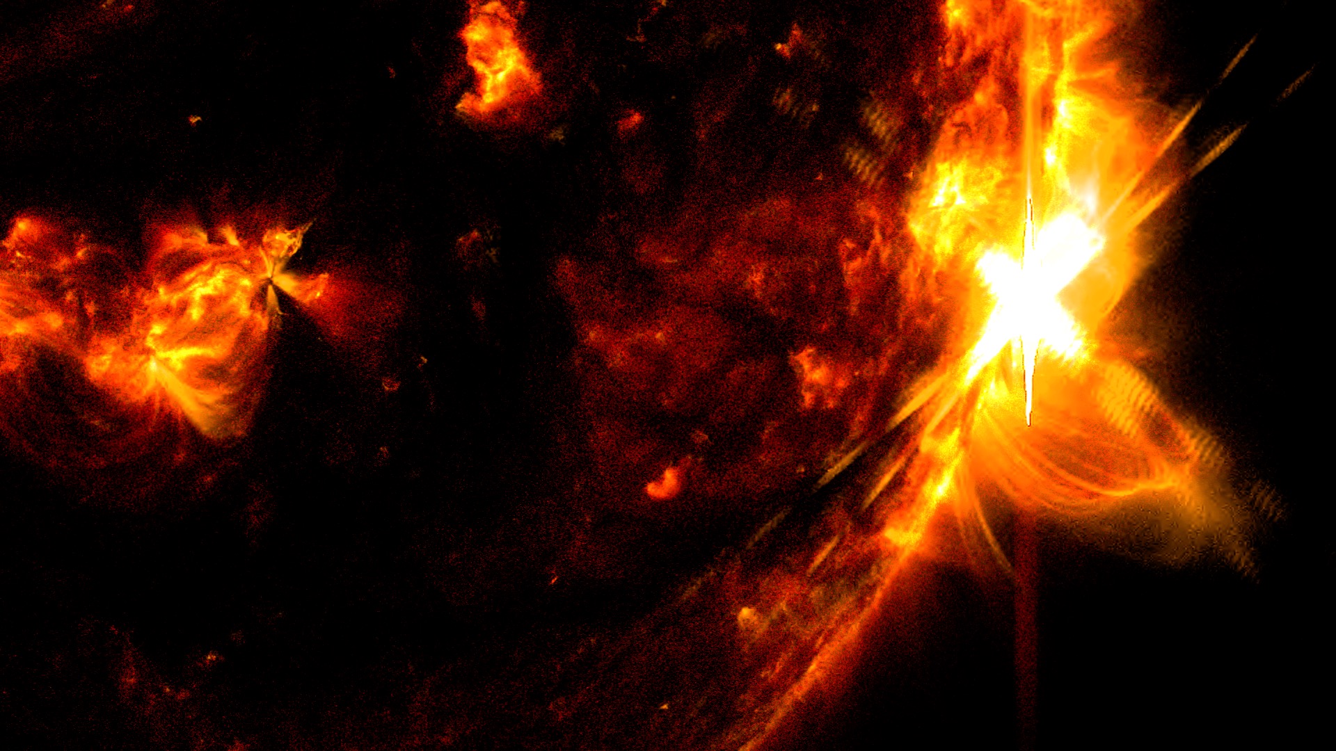
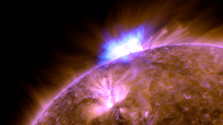
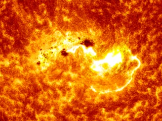
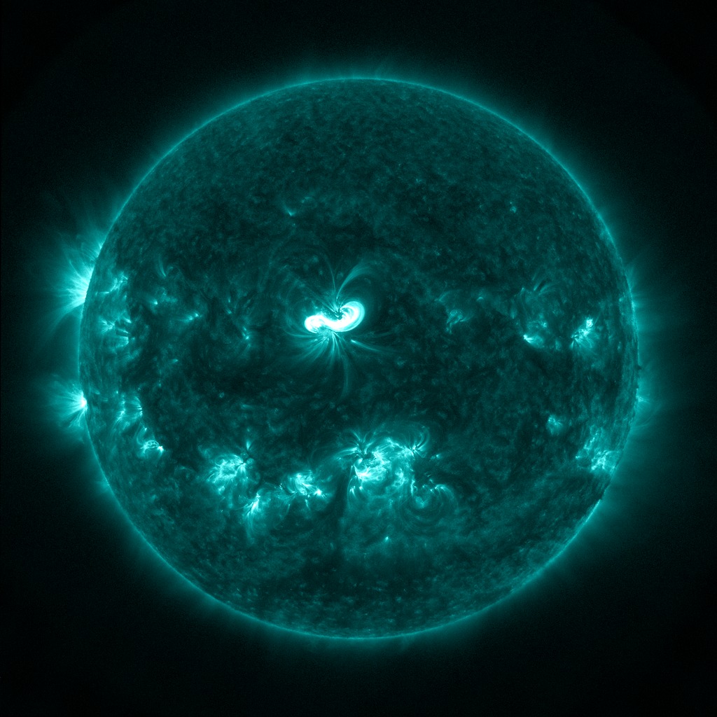
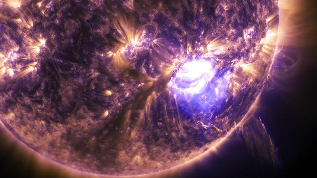
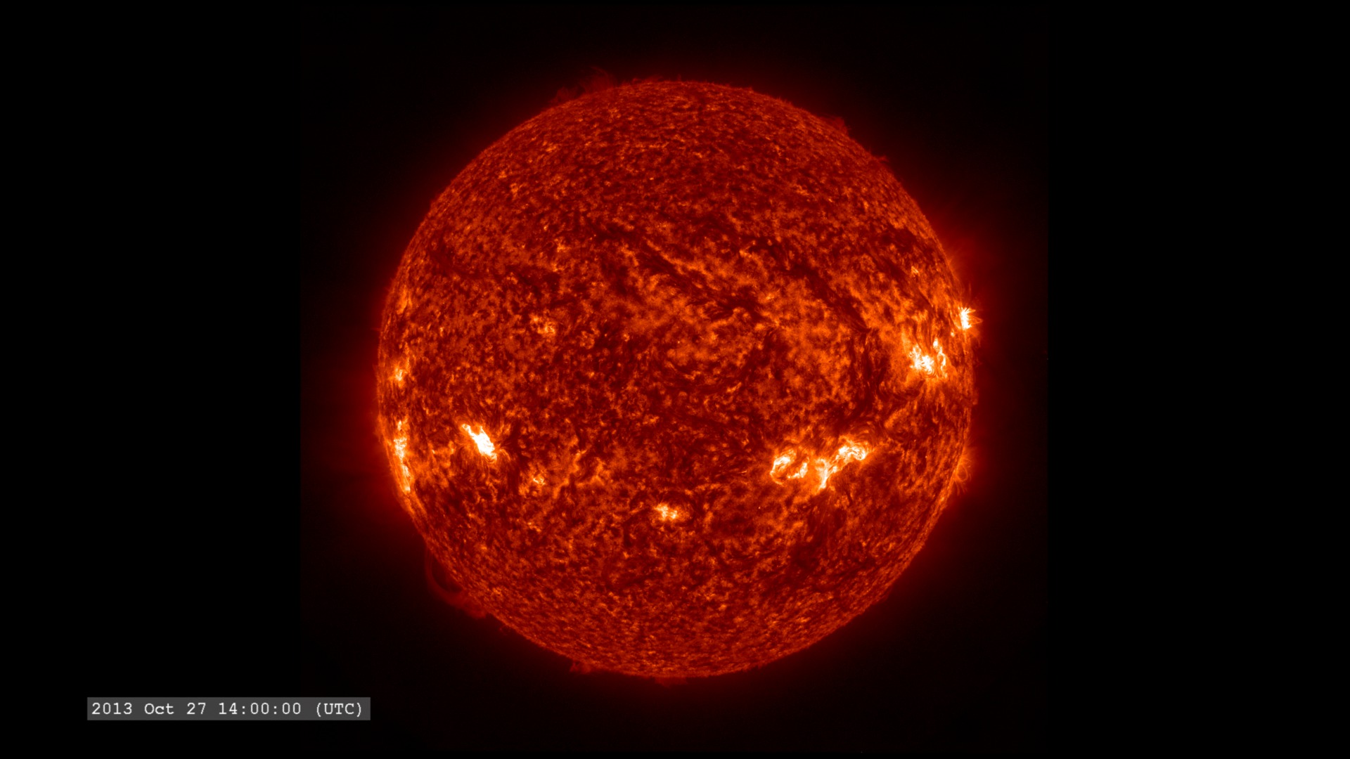
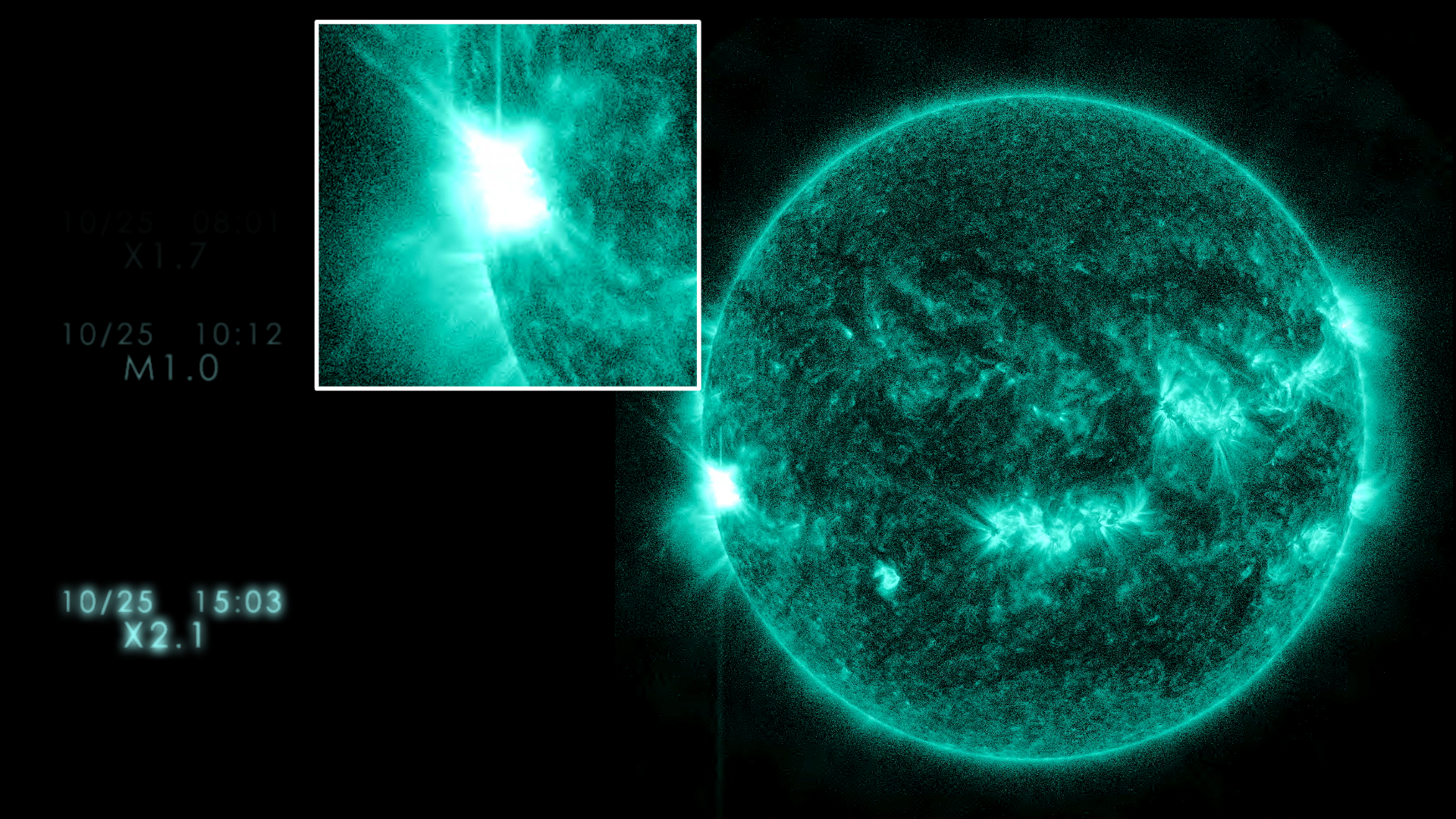
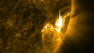
Active October Sun Emits X-class Flare
Go to this pageBrighter than a shimmering ghost, faster than the flick of a black cat’s tail, the Sun cast a spell in our direction, just in time for Halloween. This imagery captured by NASA’s Solar Dynamics Observatory covers a busy few days of activity between Oct. 25-28 that ended with a significant solar flare. From late afternoon Oct. 25 through mid-morning Oct. 26, an active region on the left limb of the Sun flickered with a series of small flares and petal-like eruptions of solar material. Meanwhile, the Sun was sporting more active regions at its lower center, directly facing Earth. On Oct. 28, the biggest of these released a significant flare, which peaked at 11:35 a.m. EDT. Credit: NASA/GSFC/SDOMusic: "Immersion" from Above and Below. Written and produced by Lars LeonhardWatch this video on the NASA Goddard YouTube channel.Complete transcript available. || ActiveOctober_Still.jpg (1920x1080) [956.2 KB] || 13982_ActiveOctober_ProRes_1920x1080_2997.mov (1920x1080) [2.4 GB] || 13982_ActiveOctober_1080_Best.mp4 (1920x1080) [436.2 MB] || 13982_ActiveOctober_1080.mp4 (1920x1080) [188.1 MB] || 13982_ActiveOctober_1080_Best.webm (1920x1080) [19.7 MB] || 13982_ActiveOctober_SRT_Captions.en_US.srt [574 bytes] || 13982_ActiveOctober_SRT_Captions.en_US.vtt [587 bytes] ||
2020
- Section
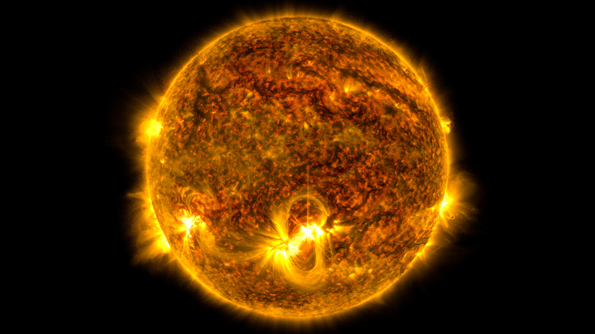
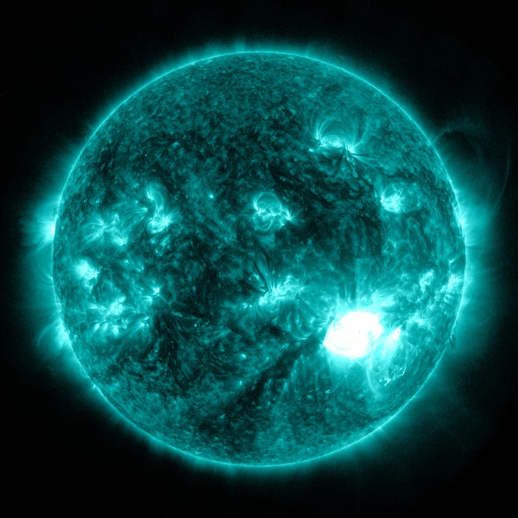
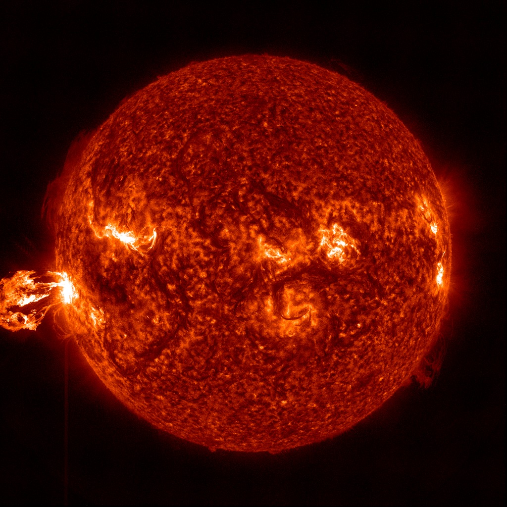
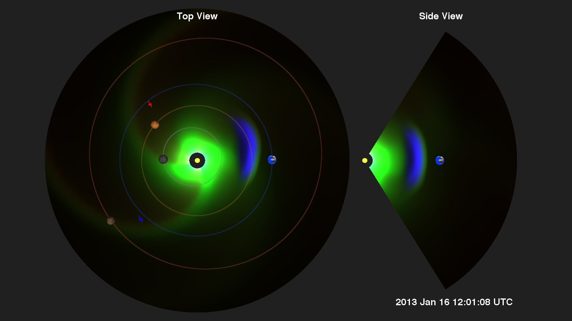
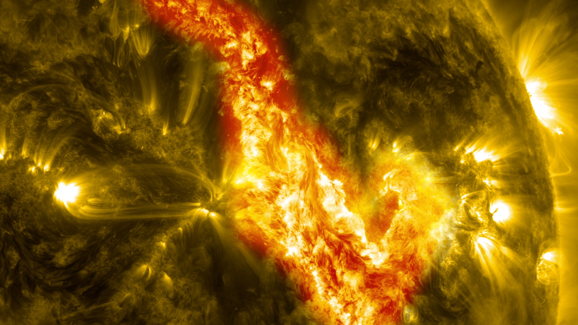
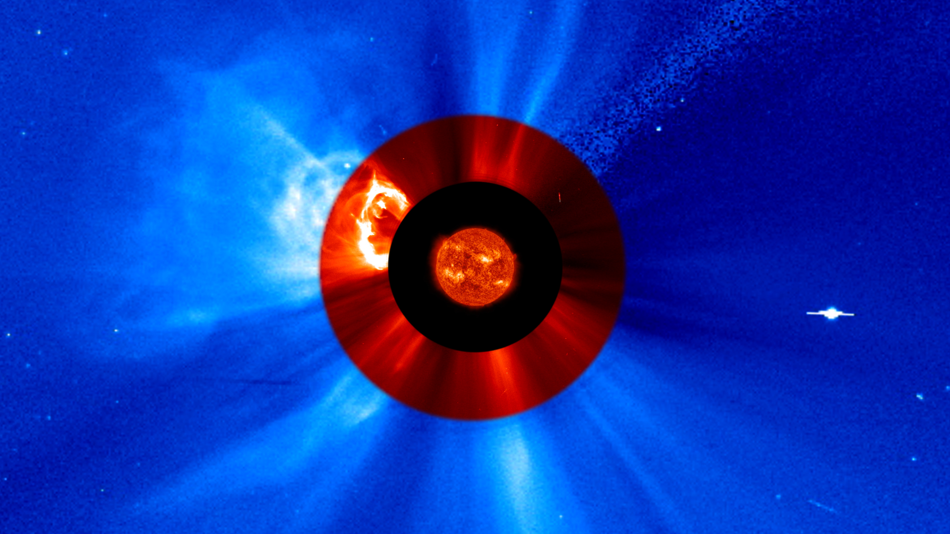
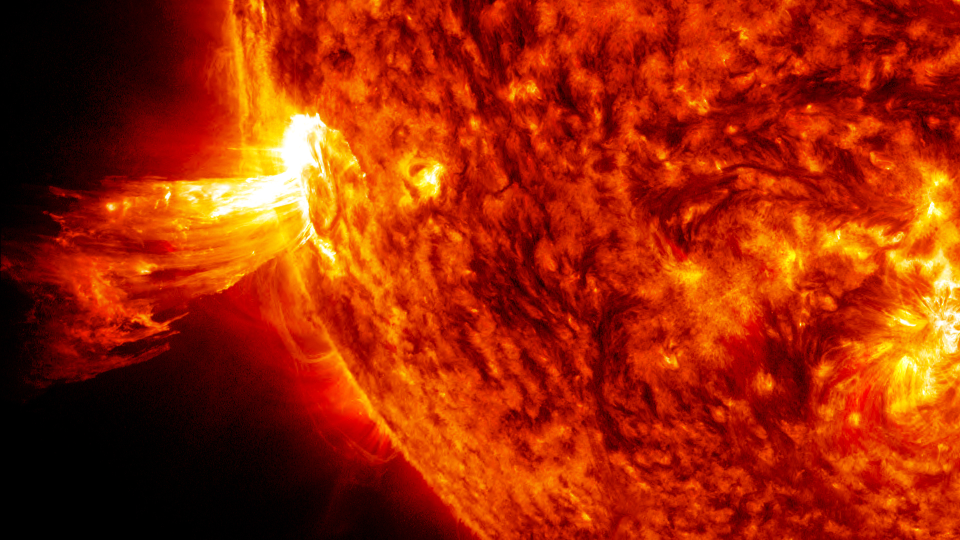
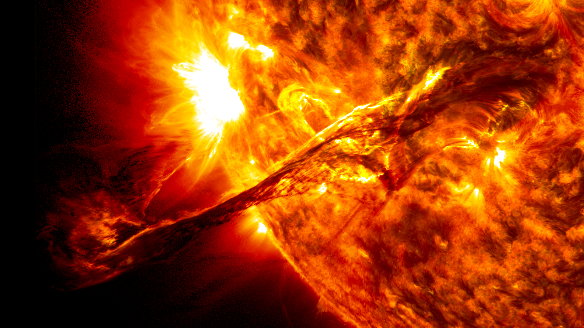
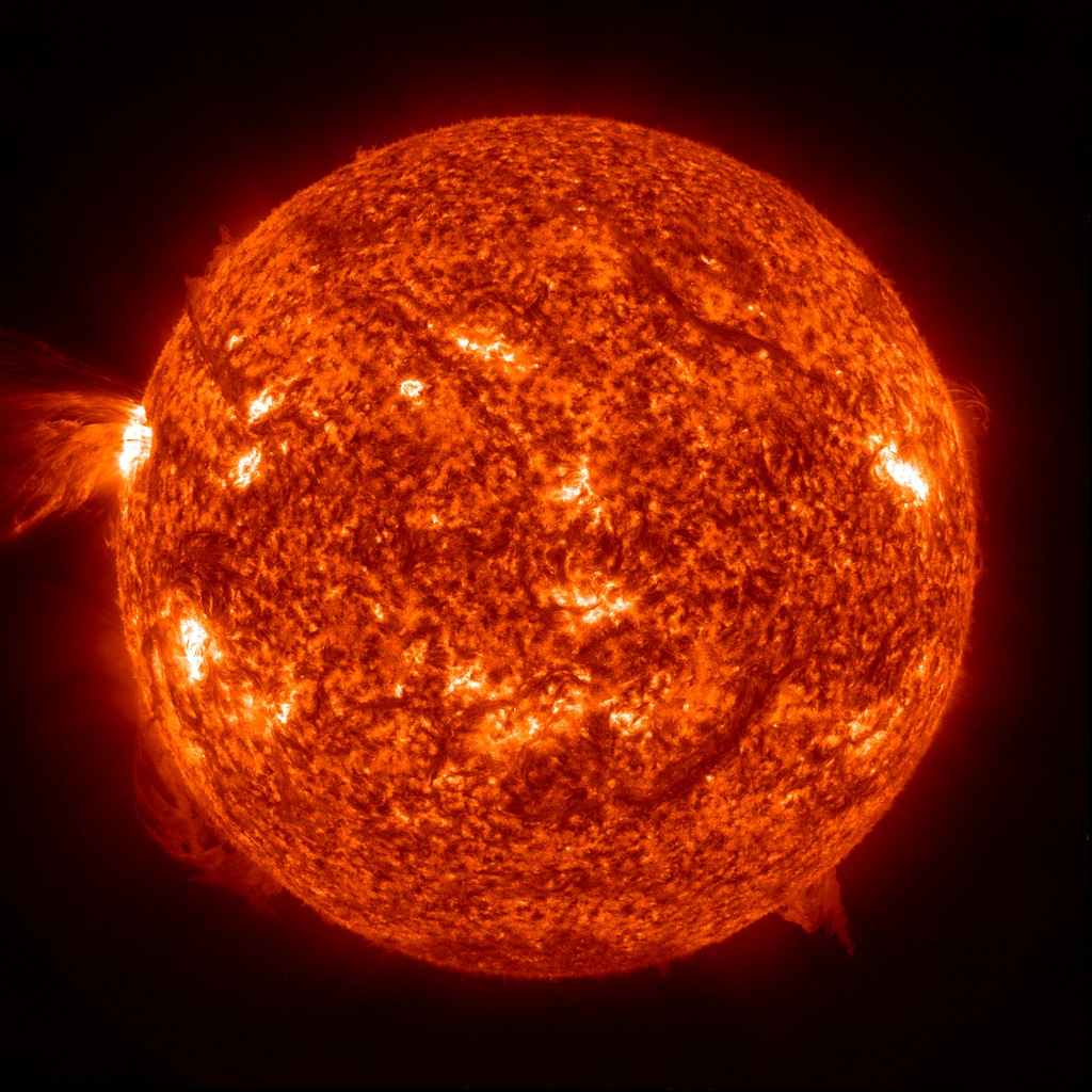
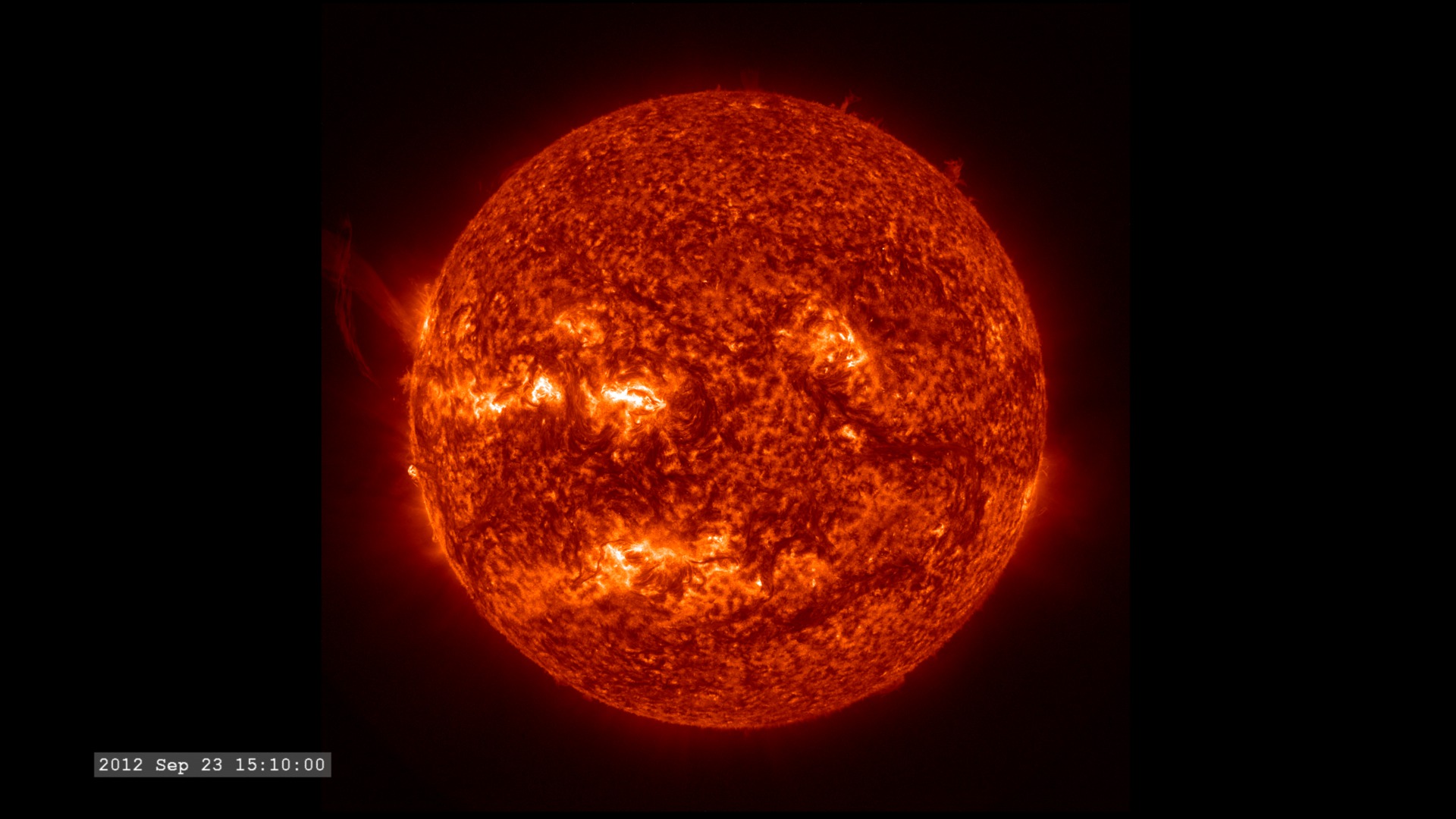
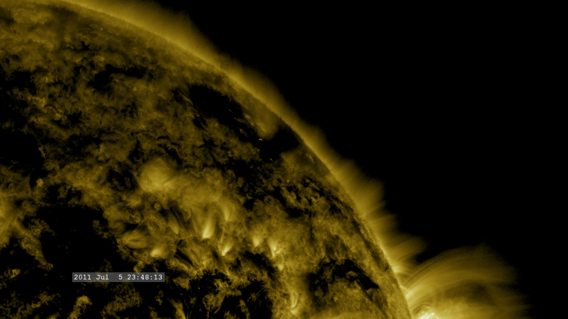
Solar Activity Continues to Rise with 'Anemone' Eruption
Go to this sectionThis imagery captured by NASA’s Solar Dynamics Observatory shows a solar flare and a subsequent eruption of solar material that occurred over the left limb of the Sun on November 29, 2020. From its foot point over the limb, some of the light and energy was blocked from reaching Earth – a little like seeing light from a lightbulb with the bottom half covered up. Also visible in the imagery is an eruption of solar material that achieved escape velocity and moved out into space as a giant cloud of gas and magnetic fields known as a coronal mass ejection, or CME. A third, but invisible, feature of such eruptive events also blew off the Sun: a swarm of fast-moving solar energetic particles. Such particles are guided by the magnetic fields streaming out from the Sun, which, due to the Sun’s constant rotation, point backwards in a big spiral much the way water comes out of a spinning sprinkler. The solar energetic particles, therefore, emerging as they did from a part of the Sun not yet completely rotated into our view, traveled along that magnetic spiral away from Earth toward the other side of the Sun. While the solar material didn’t head toward Earth, it did pass by some spacecraft: NASA’s Parker Solar Probe, NASA’s STEREO and ESA/NASA’s Solar Orbiter. Equipped to measure magnetic fields and the particles that pass over them, we may be able to study fast-moving solar energetic particles in the observations once they are downloaded. These sun-watching missions are all part of a larger heliophysics fleet that help us understand both what causes such eruptions on the Sun -- as well as how solar activity affects interplanetary space, including near Earth, where they have the potential to affect astronauts and satellites.
- ID: 4854 Visualization
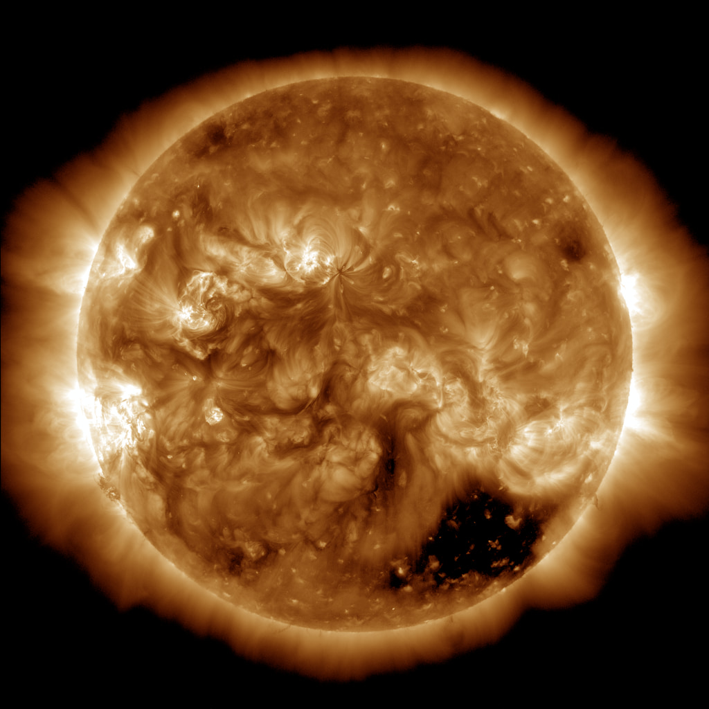
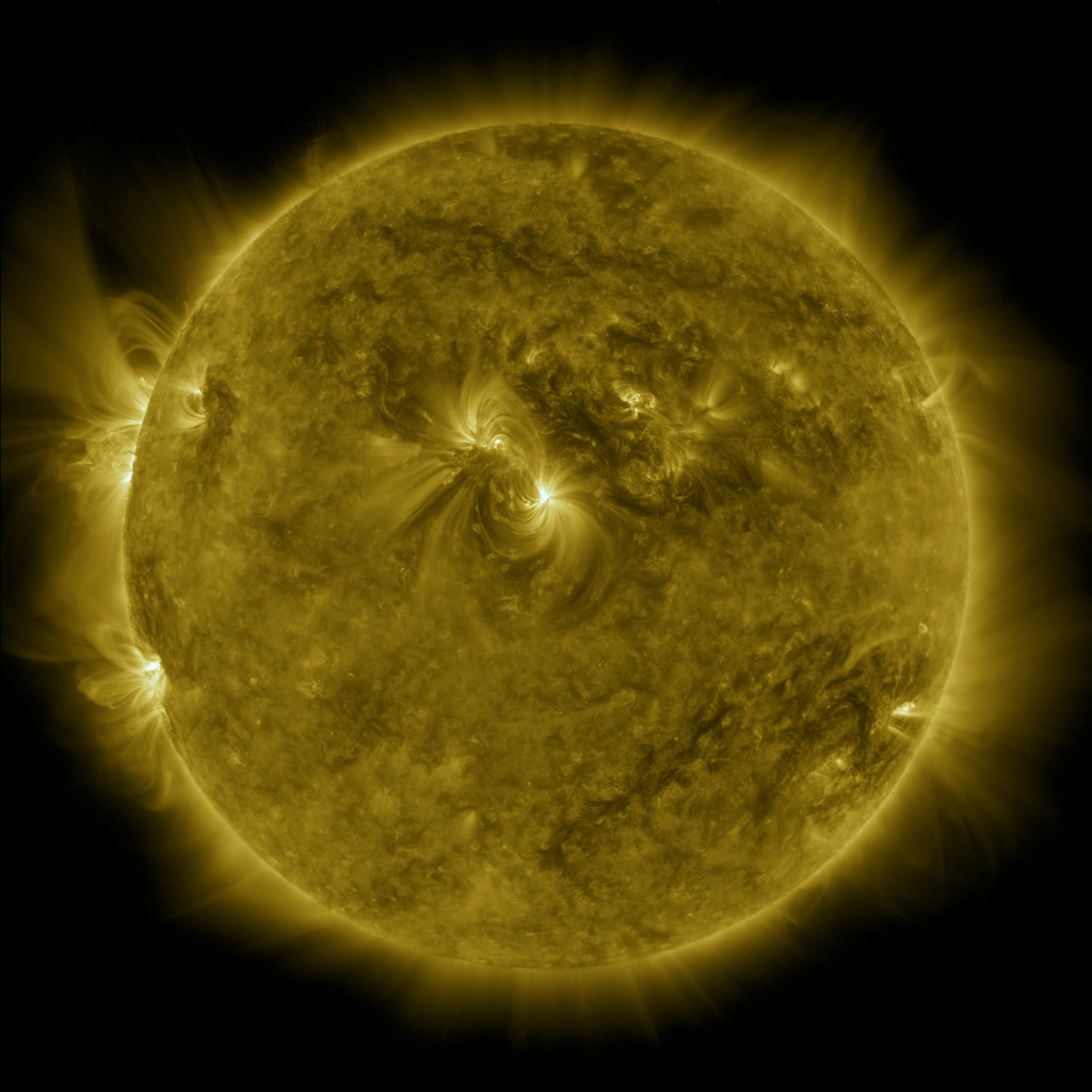
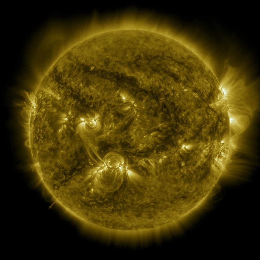
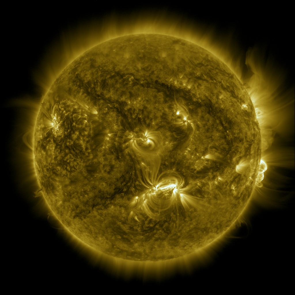
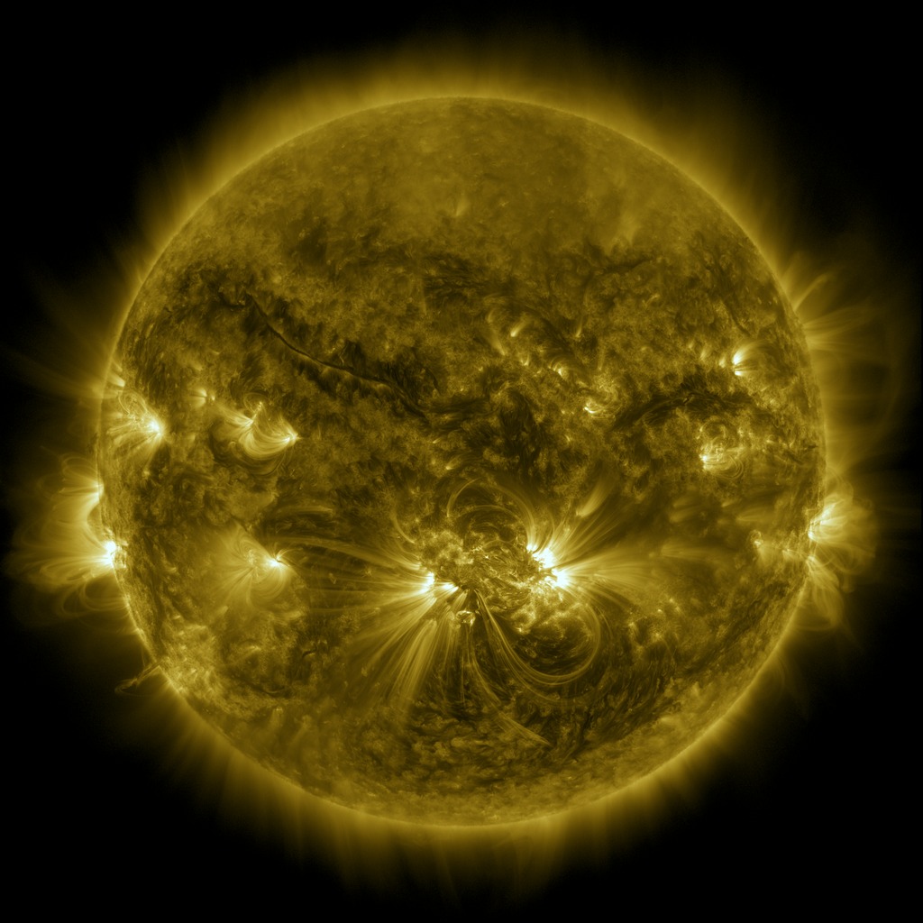
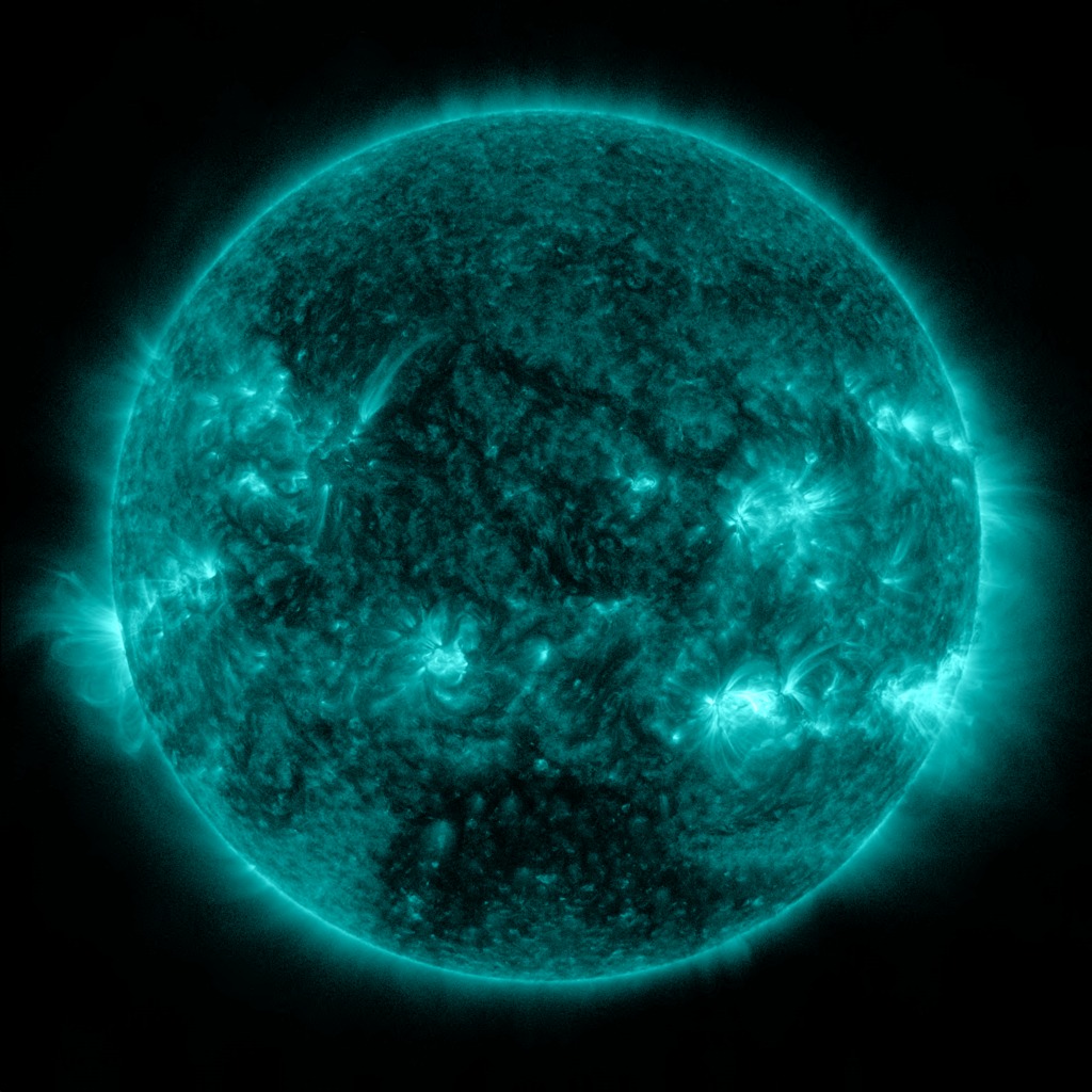
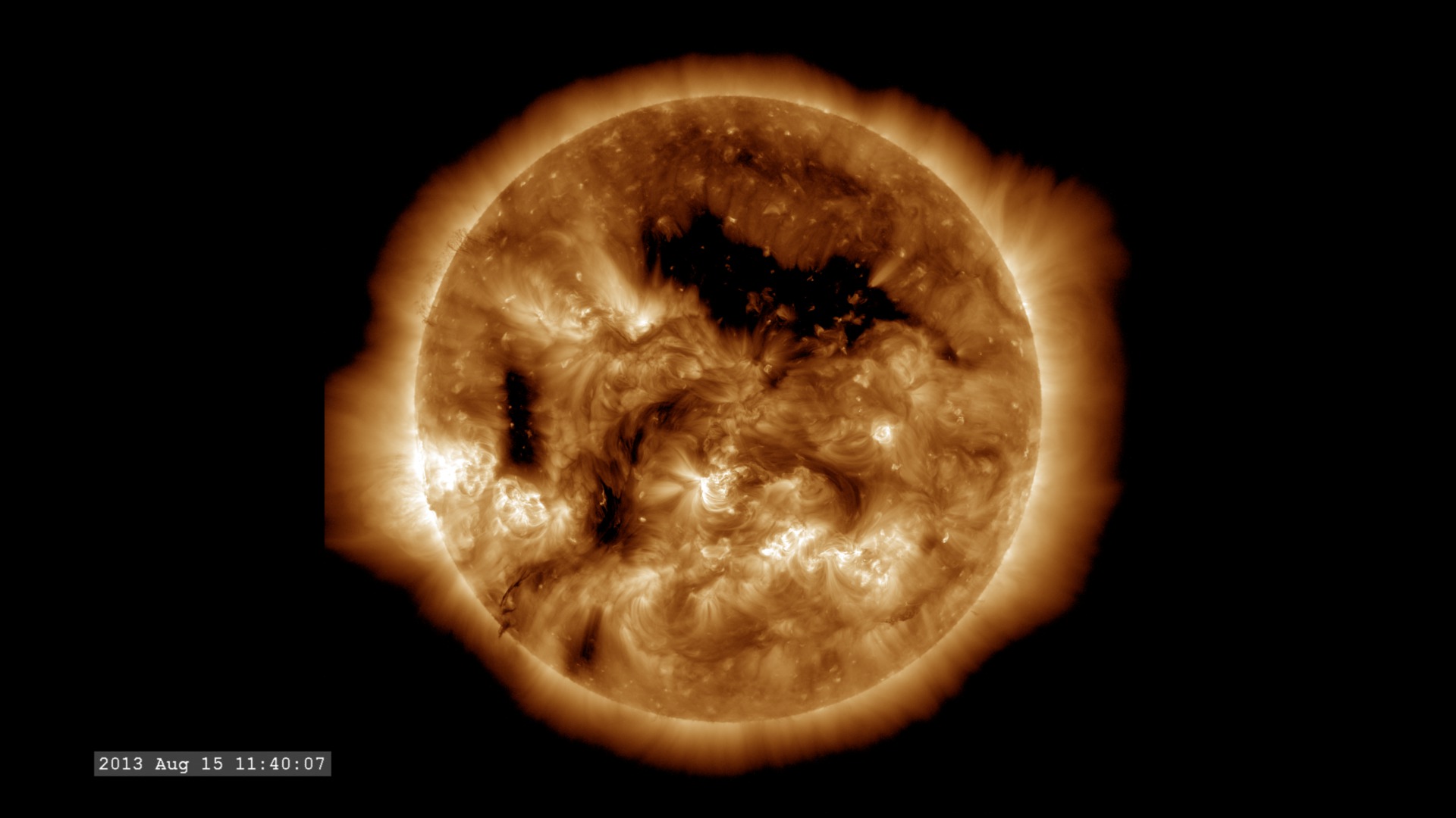
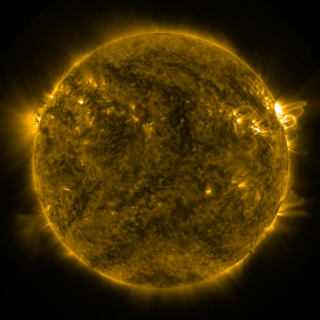
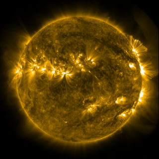
Coronal Holes at Solar Minimum and Solar Maximum
Go to this pageA sample of solar coronal holes around the time of the maximum of sunspot activity (April 2014). Note the polar regions are devoid of coronal holes but a large hole appears in the southern hemisphere. || CoronalHoleMax_AIA193_00150_print.jpg (1024x1024) [173.1 KB] || CoronalHoleMax_AIA193_00150_searchweb.png (320x180) [89.6 KB] || CoronalHoleMax_AIA193_00150_thm.png (80x40) [7.4 KB] || CoronalHoleMax_AIA193_2048p30.mp4 (2048x2048) [61.7 MB] || CoronalHoleMax_AIA193_2048p30.webm (2048x2048) [2.9 MB] || AIA193-Time (4096x4096) [64.0 KB] || AIA193-Frames (4096x4096) [64.0 KB] || CoronalHoleMax_Timestamp (600x100) [64.0 KB] ||
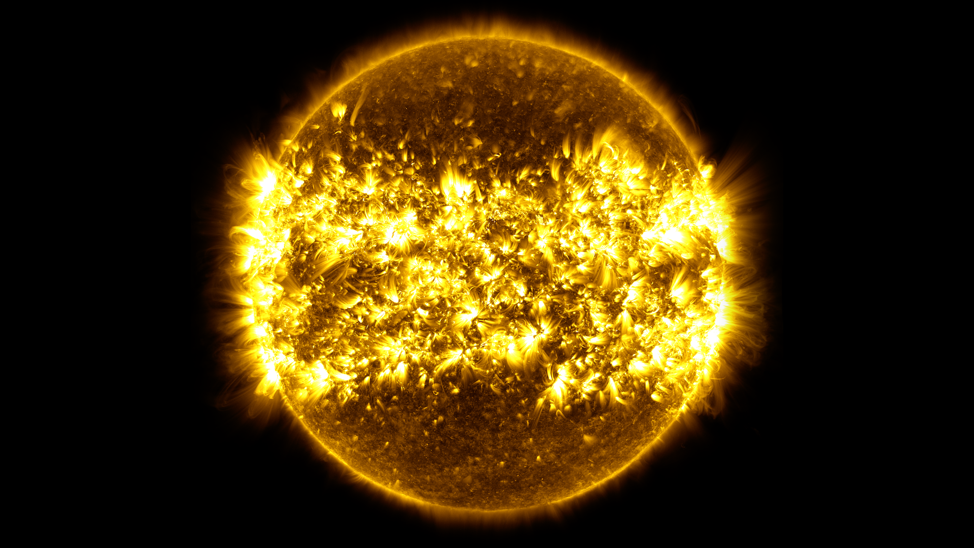
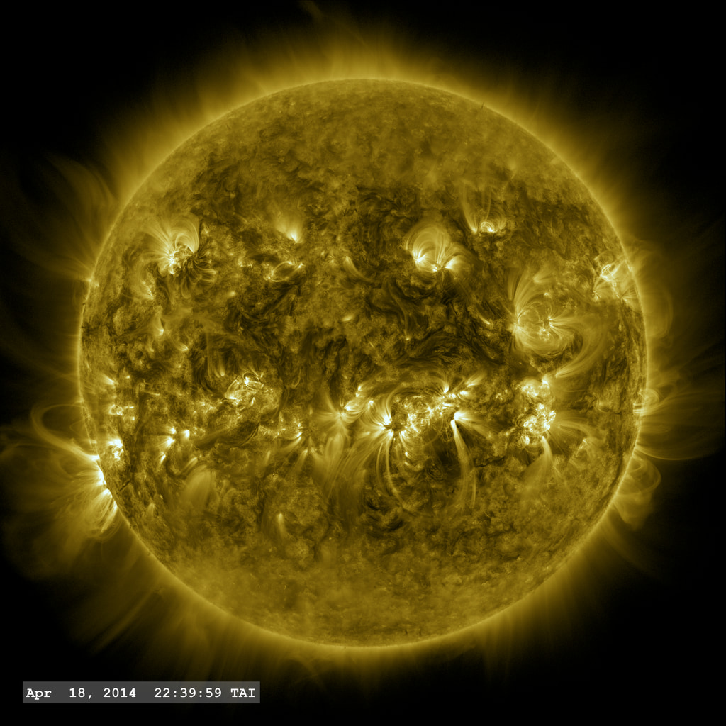
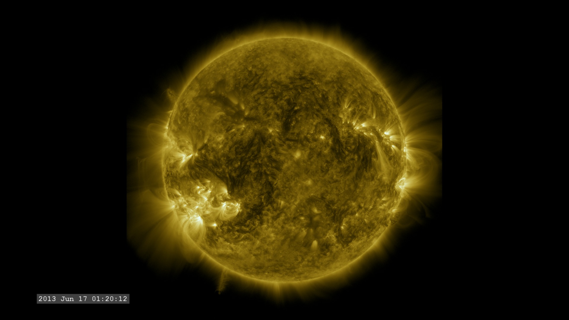
- ID: 4776 Visualization
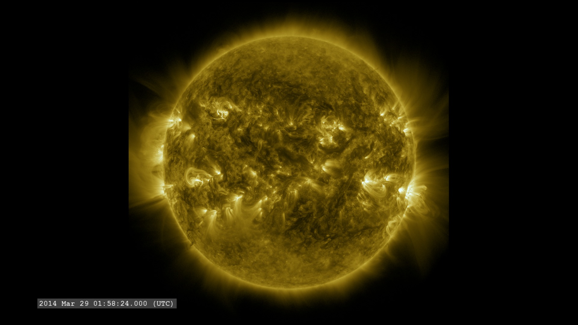
Ten Years of Solar Dynamics Observatory
Go to this pageTen years of SDO AIA 171 angstrom data with day time stamp overlay. Frames are sampled approximately one image every hour. || SDOat10_AIA171_stand.UHD2160.01500_print.jpg (1024x576) [47.4 KB] || SDOat10_AIA171_stand.UHD2160.01500_searchweb.png (320x180) [40.9 KB] || SDOat10_AIA171_stand.UHD2160.01500_thm.png (80x40) [4.0 KB] || SDOat10_AIA171.1080p30.webm (1920x1080) [348.5 MB] || SDOat10_AIA171.baseimage (3840x2160) [0 Item(s)] || SDOat10_AIA171.1080p30.mp4 (1920x1080) [3.9 GB] || SDOat10_AIA171.UHD2160_p30.mp4 (3840x2160) [13.0 GB] || SDOat10_AIA171.1080p30.mp4.hwshow [188 bytes] ||
2019
- ID: 4763 Visualization
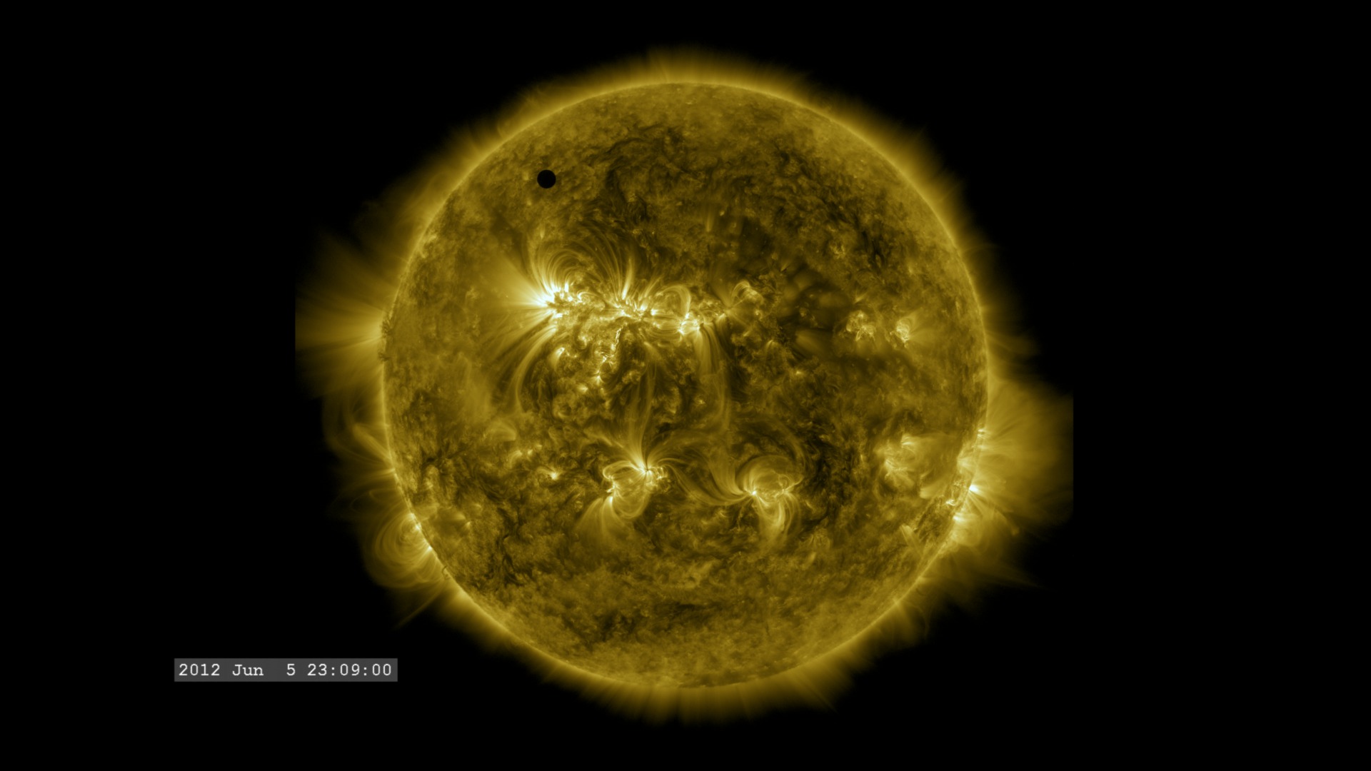
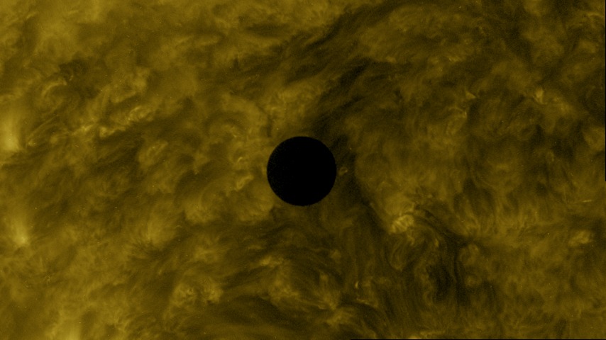
Mercury Transit, 2019 (SDO 4K imagery)
Go to this pageMercury transit visible through the 171 angstrom filter on SDO. || AIA171_00025_print.jpg (1024x1024) [108.7 KB] || AIA171_00025_searchweb.png (320x180) [65.6 KB] || AIA171_00025_thm.png (80x40) [5.2 KB] || AIA171_2048p30.mp4 (2048x2048) [19.2 MB] || AIA171_1024p30.mp4 (1024x1024) [3.7 MB] || AIA171-Frames (4096x4096) [0 Item(s)] || AIA171-Time (4096x4096) [0 Item(s)] || AIA171_4096p30_h265.mp4 (4096x4096) [13.6 MB] || AIA171_4096p30_h265.webm (4096x4096) [2.7 MB] ||
- ID: 4761 Visualization
New sites for magnetic reconnection
Go to this pageHD and UHD movie views of the plasma flowing along magnetic fields lines visible at 171Å. || May2012_Reconn_171A_stand.HD1080i.00951_print.jpg (1024x576) [52.0 KB] || May2012_Reconn_171A_stand.HD1080i.00951_searchweb.png (320x180) [43.5 KB] || May2012_Reconn_171A_stand.HD1080i.00951_thm.png (80x40) [4.2 KB] || AIA171A (1920x1080) [0 Item(s)] || May2012_Reconn_171A.HD1080i_p30.mp4 (1920x1080) [21.9 MB] || May2012_Reconn_171A.HD1080i_p30.webm (1920x1080) [7.0 MB] || AIA171A (3840x2160) [0 Item(s)] || May2012_Reconn_171A_2160p30.mp4 (3840x2160) [107.3 MB] || May2012_Reconn_171A.HD1080i_p30.mp4.hwshow [197 bytes] ||
2018
- ID: 4659 Visualization
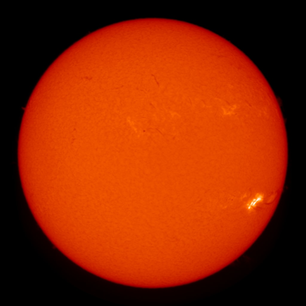
Incredible Solar Flare, Prominence Eruption and CME Event (hydrogen alpha filter)
Go to this pageThis movie is generated from imagery collected by the NSO GONG network of solar observatories. It is not time-synchronized to the related observations by the Solar Dynamics Observatory (SDO). || BBSO_Halpha_2011JuneUh_stand.HD1080i.00187_print.jpg (1024x576) [25.1 KB] || BBSO_Halpha_2011JuneUh_stand.HD1080i.00187_searchweb.png (320x180) [20.9 KB] || BBSO_Halpha_2011JuneUh_stand.HD1080i.00187_thm.png (80x40) [2.3 KB] || 1920x1080_16x9_30p (1920x1080) [0 Item(s)] || BBSO_Halpha_2011JuneUh_HD1080i_p30.mp4 (1920x1080) [2.8 MB] || BBSO_Halpha_2011JuneUh_HD1080i_p30.webm (1920x1080) [1.2 MB] || 3840x2160_16x9_30p (3840x2160) [0 Item(s)] || BBSO_Halpha_2011JuneUh_2160p30.mp4 (3840x2160) [11.4 MB] || BBSO_Halpha_2011JuneUh_HD1080i_p30.mp4.hwshow [200 bytes] ||
2017
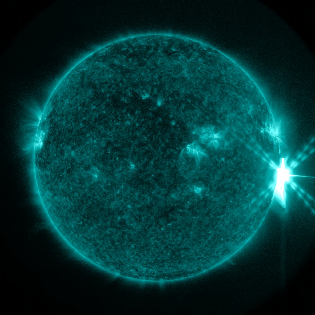
- ID: 4491 Visualization
The X8.2 Flare of September 2017, as Seen by SDO
Go to this page40 hours of AIA 131 angstrom imager at 12 second cadence viewing the time around the X8.2 solar flare. || Sept2017_X8Flare_131A_stand.UHD3840.07800_print.jpg (1024x576) [61.1 KB] || AIA131A (1920x1080) [0 Item(s)] || Sept2017_X8Flare_131A.HD1080i_p30.webm (1920x1080) [47.6 MB] || Sept2017_X8Flare_131A.HD1080i_p30.mp4 (1920x1080) [843.8 MB] || AIA131A (3840x2160) [0 Item(s)] || Sept2017_X8Flare_131A.HD1080i_p30.mp4.hwshow ||
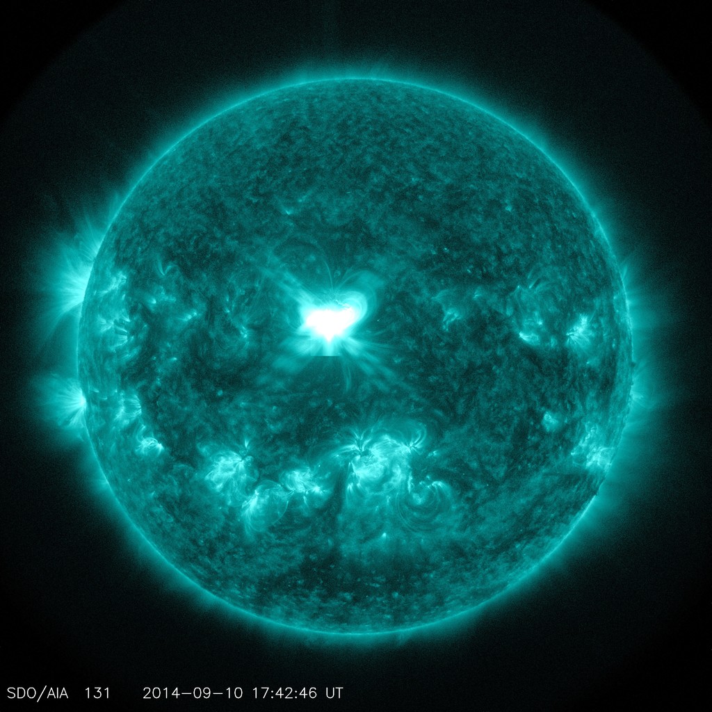
- ID: 12737 Produced Video
September Flares 4k
Go to this page4k frames and ProRes video from SDO quicklook products. This footage is in 131 angstrom extreme ultraviolet light at approximately 30 second imaging cadence. It covers the time period of 14:59 to 17:00UTC 9/10/2017. || SDO_20170910_131_AR12673X8.00680_print.jpg (1024x1024) [220.6 KB] || SDO_20170910_131_AR12673X8.00680_searchweb.png (180x320) [55.4 KB] || SDO_20170910_131_AR12673X8.00680_thm.png (80x40) [4.7 KB] || SDO_20170910_131_AR12673X8_4k.mov (4096x4096) [958.7 MB] || 131X8 (4096x4096) [16.0 KB] || SDO_20170910_131_AR12673X8_4k.webm (4096x4096) [37.1 MB] || SDO_20170910_131_AR12673X8.00680.tif (4096x4096) [12.7 MB] ||
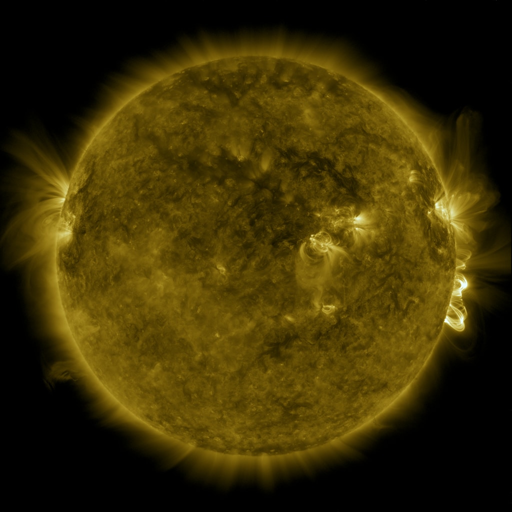
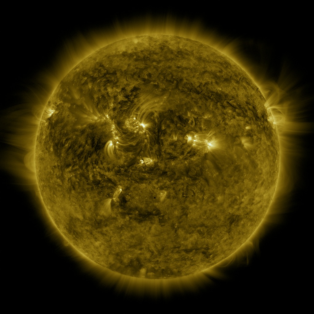
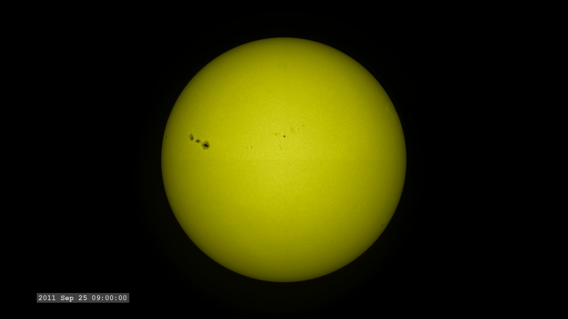
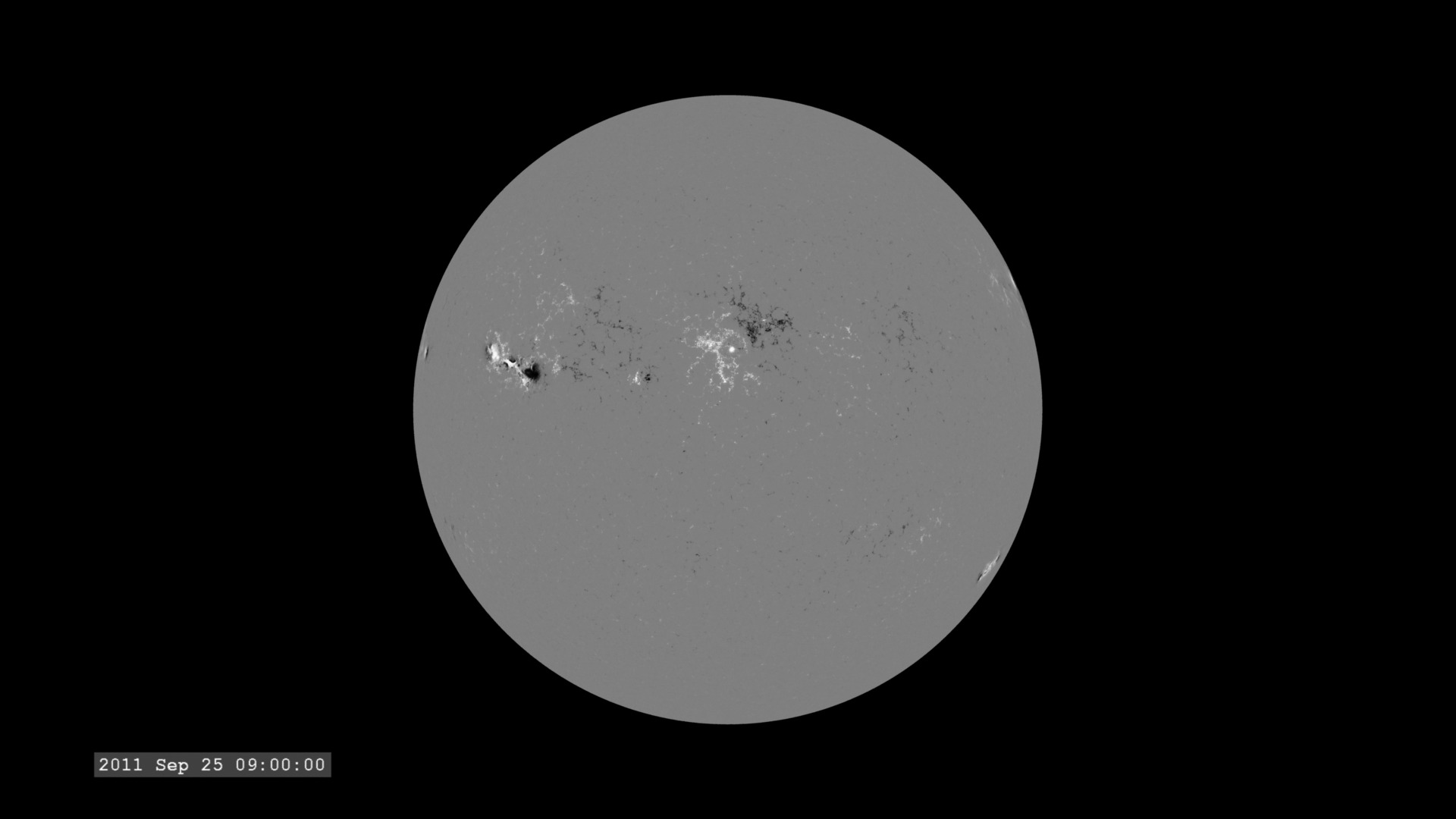
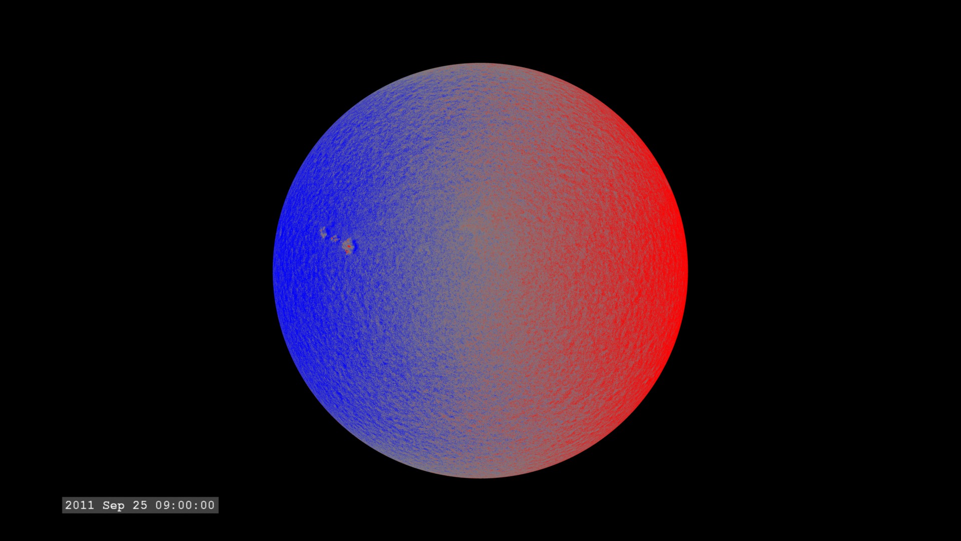
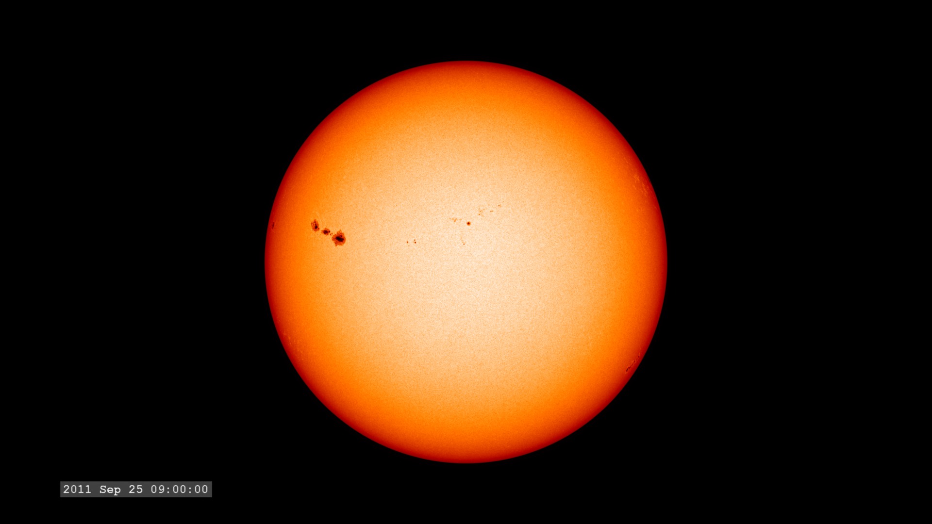
- ID: 4551 Visualization
A Solar Cycle from Solar Dynamics Observatory
Go to this page4K x 4K imagery from the SDO/HMI instrument. || SolarCycleHMI.02000_print.jpg (1024x1024) [154.4 KB] || SolarCycleHMI.02000_searchweb.png (320x180) [50.4 KB] || SolarCycleHMI.02000_thm.png (80x40) [3.7 KB] || SolarCycleHMI_1024p30.mp4 (1024x1024) [333.3 MB] || SolarCycleHMI_1024p30.webm (1024x1024) [19.2 MB] || Intensity-Frames (4096x4096) [512.0 KB] || Intensity-Time (4096x4096) [512.0 KB] ||
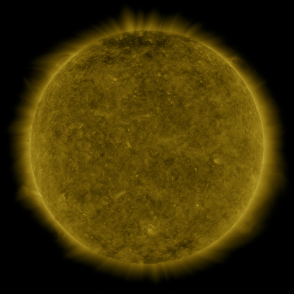
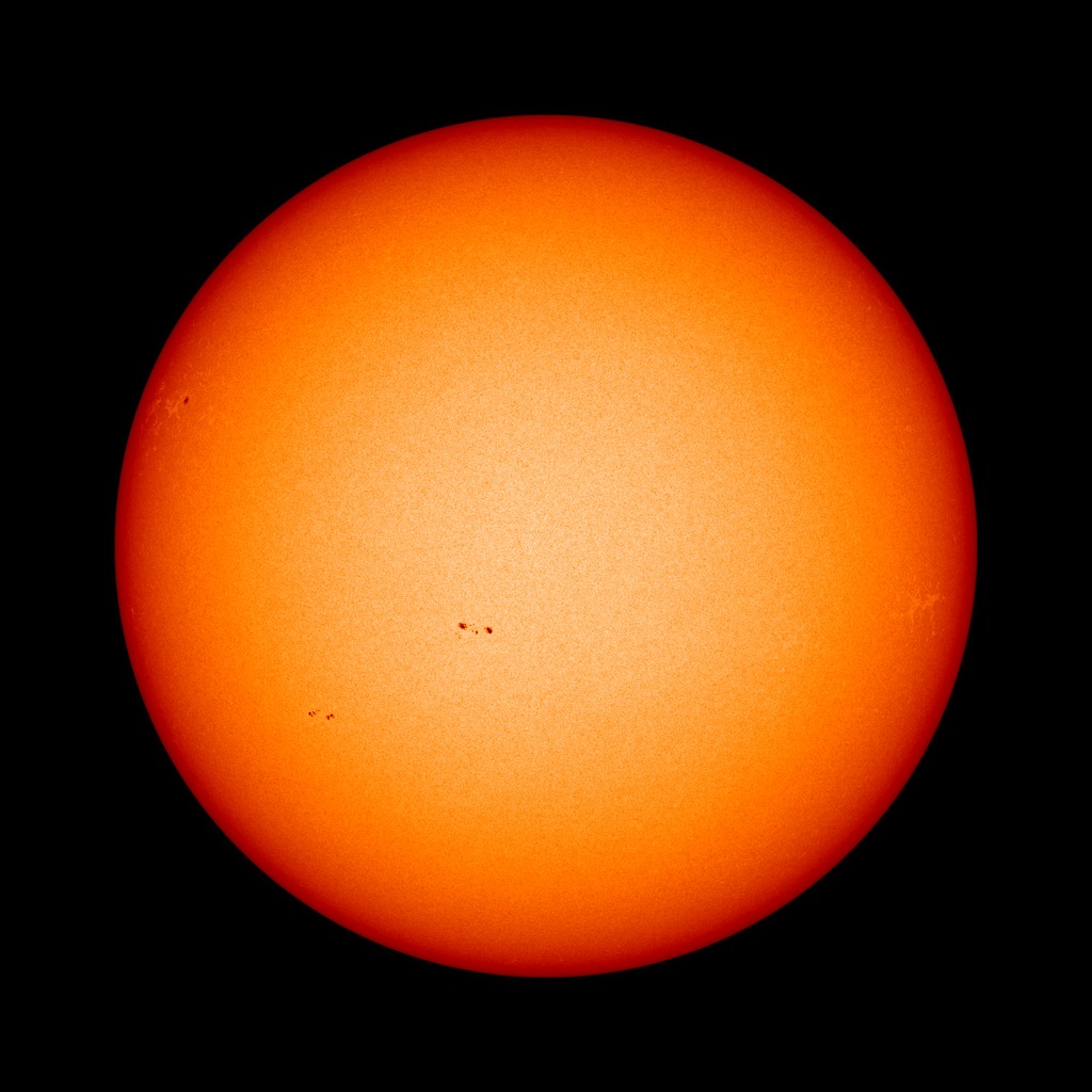
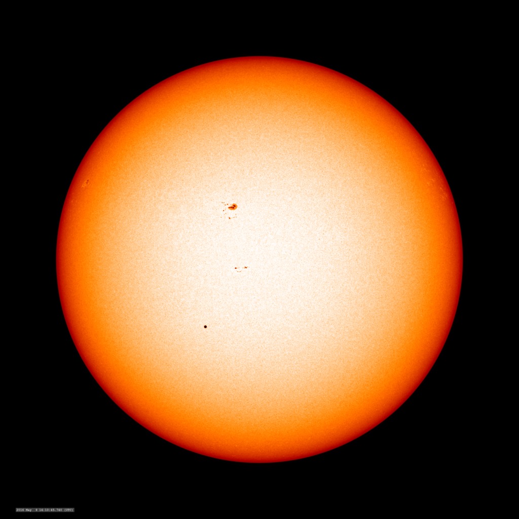
- ID: 4002 Visualization
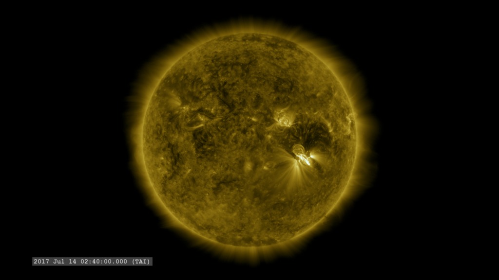
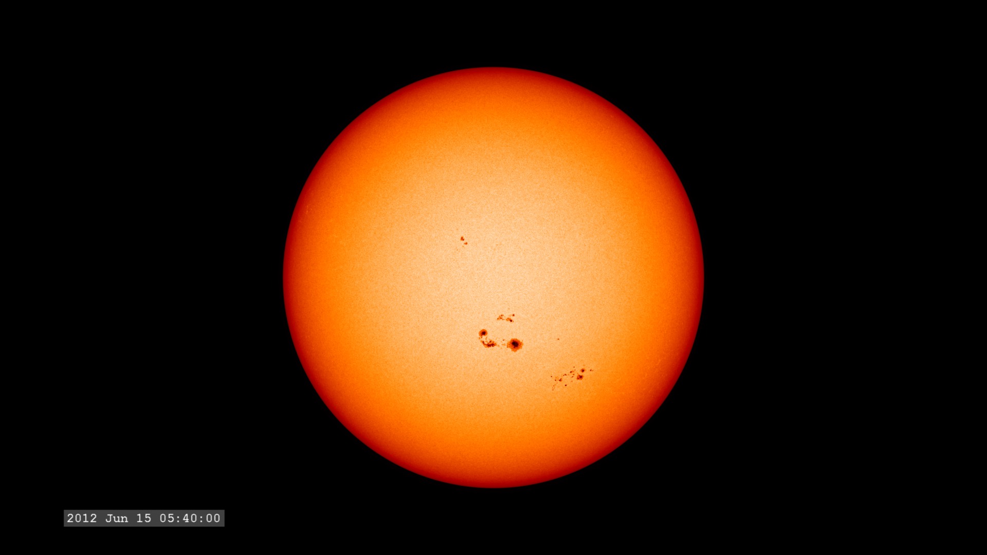
AR2665: The Lonely Sunspot of Solar Minimum
Go to this pageFull-disk view of sunspot group moving across the solar disk, AIA 171 ångstrom band. || July2017_AR2665_AIA171_stand.HD1080i.01000_print.jpg (1024x576) [53.8 KB] || AIA171 (1920x1080) [0 Item(s)] || July2017_AR2665_AIA171.HD1080i_p30.mp4 (1920x1080) [53.5 MB] || July2017_AR2665_AIA171.HD1080i_p30.webm (1920x1080) [8.5 MB] || July2017_AR2665_AIA171_2048p30.mp4 (2048x2048) [264.8 MB] || 171A-Frames (4096x4096) [0 Item(s)] || 171A-Time (4096x4096) [0 Item(s)] || July2017_AR2665_AIA171.HD1080i_p30.mp4.hwshow [200 bytes] ||
2016
- ID: 4463 Visualization

Mercury Transit 2016 from SDO/AIA at 304 Ångstroms
Go to this pageComposited full-disk imagery sampled at 12 second intervals. || AIA304MercuryComposite.01500_print.jpg (1024x1024) [195.3 KB] || AIA304MercuryComposite.01500_searchweb.png (320x180) [69.7 KB] || AIA304MercuryComposite.01500_thm.png (80x40) [4.7 KB] || AIA304MercuryComposite_2048p30.webm (720x720) [9.5 MB] || AIA304MercuryComposite_2048p30.mp4 (2048x2048) [597.8 MB] || 304A-Frames (4096x4096) [0 Item(s)] || 304A-Time (4096x4096) [0 Item(s)] ||
- ID: 4462 Visualization
Mercury Transit 2016 from SDO/AIA at 171 Ångstroms
Go to this pageComposited full-disk imagery sampled at 12 second intervals. || AIA171MercuryComposite.01500_print.jpg (1024x1024) [187.2 KB] || AIA171MercuryComposite.01500_searchweb.png (320x180) [82.8 KB] || AIA171MercuryComposite.01500_thm.png (80x40) [6.3 KB] || aia171mercurycomposite_2048p30.webm (720x720) [6.6 MB] || AIA171MercuryComposite_2048p30.mp4 (2048x2048) [297.0 MB] || 171A-Frames (4096x4096) [0 Item(s)] || 171A-Time (4096x4096) [0 Item(s)] ||
- ID: 4461 Visualization
Mercury Transit 2016 from SDO/HMI
Go to this pageFull-Disk imagery sampled at 3 second cadence. || HMIMercuryComposite_stand.4Kx4K.04000_print.jpg (1024x1024) [141.4 KB] || HMIMercuryComposite_stand.4Kx4K.04000_searchweb.png (320x180) [50.3 KB] || HMIMercuryComposite_stand.4Kx4K.04000_thm.png (80x40) [3.9 KB] || HMIMercuryComposite_stand.2Kx2Kp30.webm (2048x2048) [30.4 MB] || HMIMercuryComposite_stand.2Kx2Kp30.mp4 (2048x2048) [637.1 MB] || 4096x4096_1x1_30p (4096x4096) [0 Item(s)] ||
- ID: 12144 Produced Video
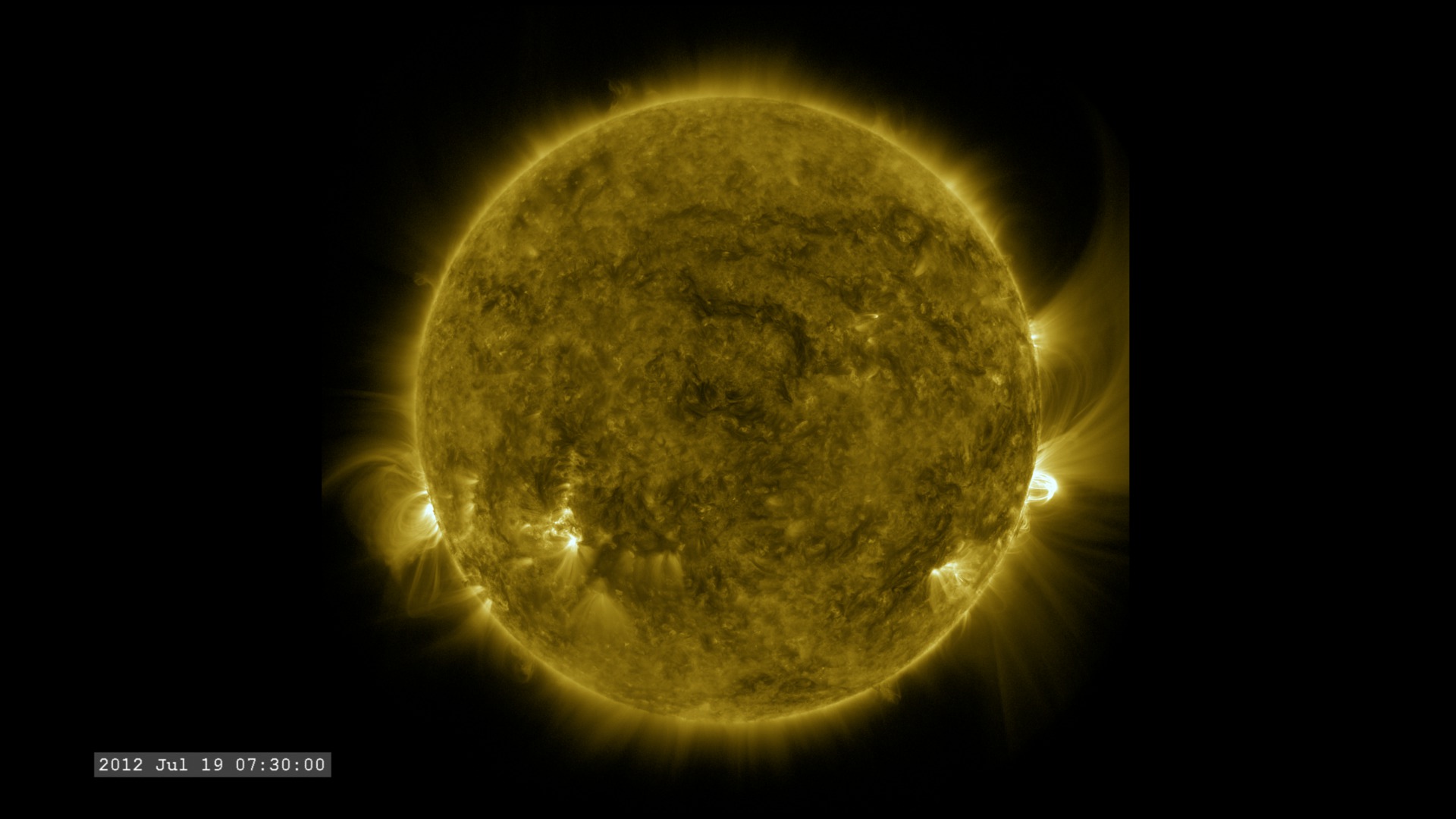
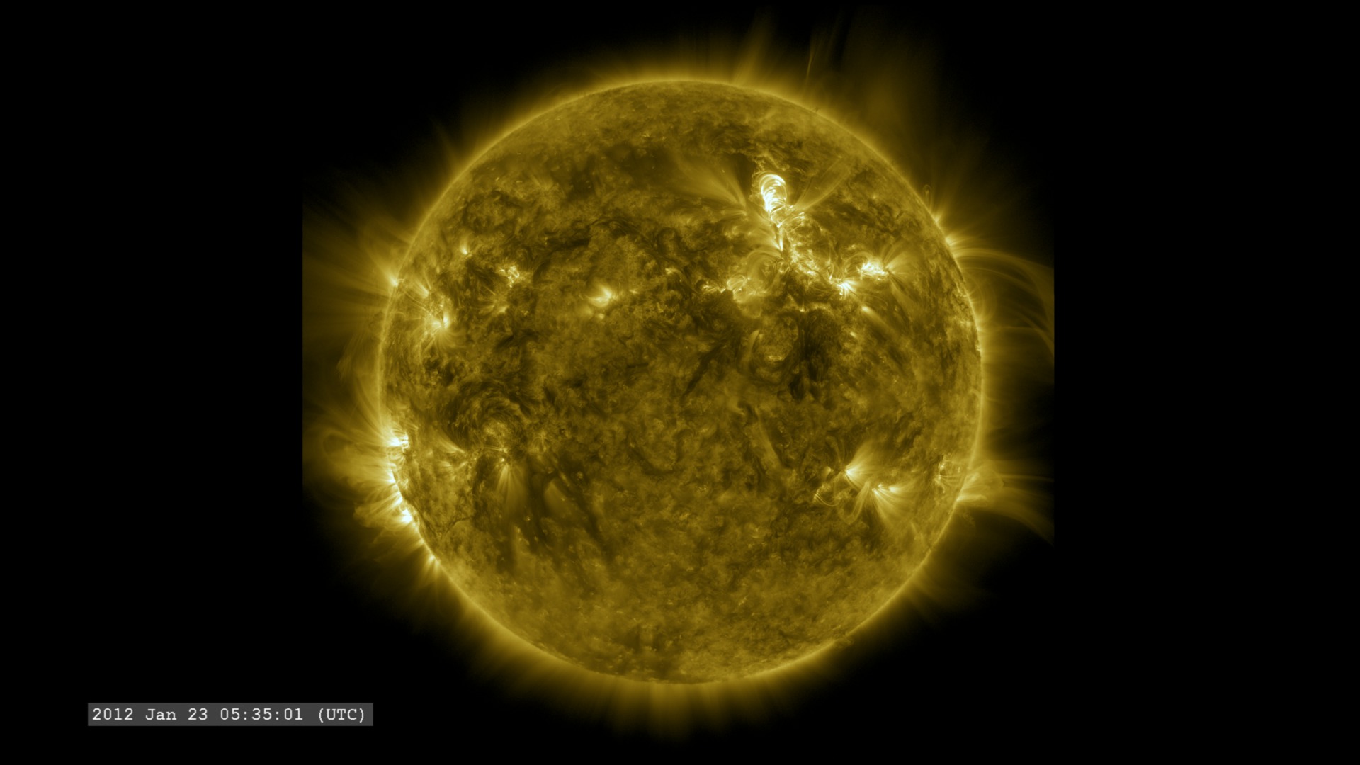
SDO: Year 6
Go to this pageThis ultra-high definition (3840x2160) video shows the sun in the 171 angstrom wavelength of extreme ultraviolet light. It covers a time period of January 2, 2015 to January 28, 2016 at a cadence of one frame every hour, or 24 frames per day. This timelapse is repeated with narration by solar scientist Nicholeen Viall and contains close-ups and annotations. 171 angstrom light highlights material around 600,000 Kelvin and shows features in the upper transition region and quiet corona of the sun. The video is available to download here at 59.94 frames per second, double the rate YouTube currently allows for UHD content. The music is titled "Tides" and is from Killer Tracks.Watch this video on the NASA Goddard YouTube channel.Complete transcript available. || SDO_Year6_HCblend_HD.png (1920x1080) [5.3 MB] || SDO_Year6_HCblend_HD.jpg (1920x1080) [545.9 KB] || SDO_Year6_HCblend_HD_print.jpg (1024x576) [179.5 KB] || SDO_Year6_HCblend_UHD.png (3840x2160) [19.7 MB] || SDO_Year6_HCblend_UHD.jpg (3840x2160) [1.2 MB] || SDO_Year6_HCblend_HD_searchweb.png (180x320) [59.6 KB] || SDO_Year6_HCblend_HD_thm.png (80x40) [4.8 KB] || 12144_SDO_Year_6_appletv.webm (1280x720) [50.5 MB] || 12144_SDO_Year_6_appletv.m4v (1280x720) [241.9 MB] || 12144_SDO_Year_6_appletv_appletv_subtitles.m4v (1280x720) [242.1 MB] || SDO_Year_6_SRT_Captions.en_US.srt [6.3 KB] || SDO_Year_6_SRT_Captions.en_US.vtt [6.3 KB] || 12144_SDO_Year_6_H264_Good_1920x1080_2997.mov (1920x1080) [1.4 GB] || 12144_SDO_Year_6_H264_Good_3840x2160_2997.mov (3840x2160) [9.1 GB] || 12144_SDO_Year_6_H264_Good_3840x2160_5994.mov (3840x2160) [10.2 GB] || 12144_SDO_Year_6_ProRes_3840x2160_5994.mov (3840x2160) [50.3 GB] ||
- ID: 4422 Visualization
SDO Year 6: A Year of the Sun
Go to this pageA year of SDO solar observations in HD1080. || SDOYear6hourly_171A_stand.HD1080i.02000_print.jpg (1024x576) [64.8 KB] || 1920x1080_16x9_30p (1920x1080) [0 Item(s)] || SDOYear6hourly_171A.HD1080.webm (1920x1080) [37.4 MB] || SDOYear6hourly_171A_1080p30.mp4 (1920x1080) [424.4 MB] || SDOYear6hourly_171A.HD1080.mov (1920x1080) [1.1 GB] || SDOYear6hourly_171A_1080p30.mp4.hwshow [193 bytes] ||
2015
- ID: 11868 Produced Video
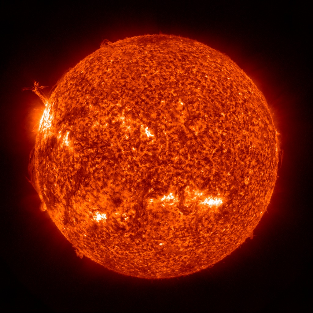
NASA's SDO Observes a Cinco de Mayo Solar Flare
Go to this pageVideo of May 5, 2015 X2.7 flare.Credit: NASA/GSFC/SDO || May_5_2015_Flare_Still_304-171.png (1920x1080) [8.1 MB] || May_5_2015_Flare_Still_304-171.jpg (1920x1080) [415.9 KB] || May_5_2015_Flare_Still_304-171_print.jpg (1024x576) [145.7 KB] || May_5_2015_Flare_Still_304-171_web.png (320x180) [83.3 KB] || 11868_May_5_X_Flare_MPEG4_1920X1080_2997.mp4 (1920x1080) [42.2 MB] || 11868_May_5_X_Flare_H264_Good_1920x1080_2997.webm (1920x1080) [4.8 MB] || 11868_May_5_X_Flare_1280x720.wmv (1280x720) [23.1 MB] || 11868_May_5_X_Flare_appletv.m4v (960x540) [19.0 MB] || 11868_May_5_X_Flare_appletv_subtitles.m4v (960x540) [19.0 MB] || 11868_May_5_X_Flare_ipod_lg.m4v (640x360) [7.1 MB] || 11868_May_5_X_Flare_ipod_sm.mp4 (320x240) [3.6 MB] || 11868_May_5_X_Flare_SRT_Captions.en_US.srt [230 bytes] || 11868_May_5_X_Flare_SRT_Captions.en_US.vtt [243 bytes] || 11868_May_5_X_Flare_ProRes_1920x1080_2997.mov (1920x1080) [674.9 MB] || 11868_May_5_X_Flare_H264_Best_1920x1080_2997.mov (1920x1080) [682.7 MB] || 11868_May_5_X_Flare_H264_Good_1920x1080_2997.mov (1920x1080) [219.1 MB] ||
- ID: 4323 Visualization
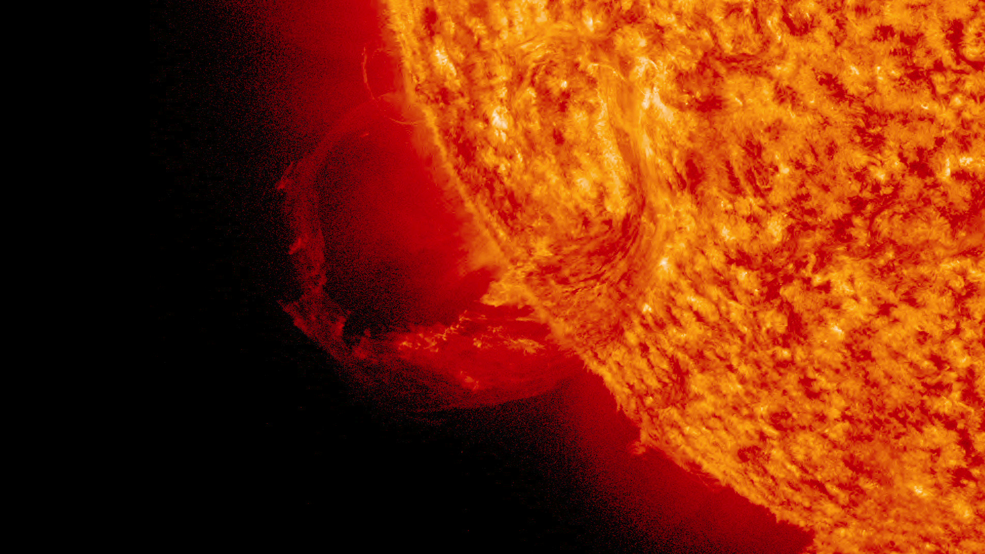
Summer Sun from SDO: Eruption and Coronal Loops on the Solar Limb
Go to this pageHD1080 movie of the Sun in the AIA 304 angstrom filter. Note the coronal loop structures on the lower right limb. || June2015LimbLoops_304A_stand.HD1080i.00256_print.jpg (1024x576) [68.0 KB] || June2015LimbLoops_304A_1080p.webm (1920x1080) [5.1 MB] || June2015LimbLoops_304AHD (1920x1080) [128.0 KB] || June2015LimbLoops_304A_1080p.mp4 (1920x1080) [34.7 MB] || June2015LimbLoops_304A.HD1080.mov (1920x1080) [108.5 MB] || June2015LimbLoops_304A_1080p.mp4.hwshow [228 bytes] ||
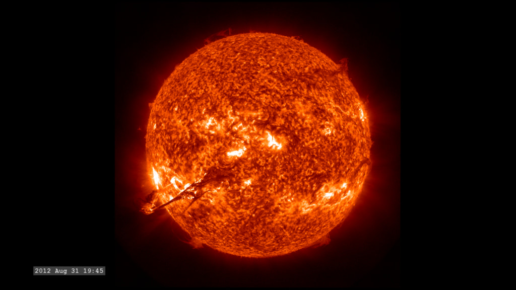
- ID: 4319 Visualization
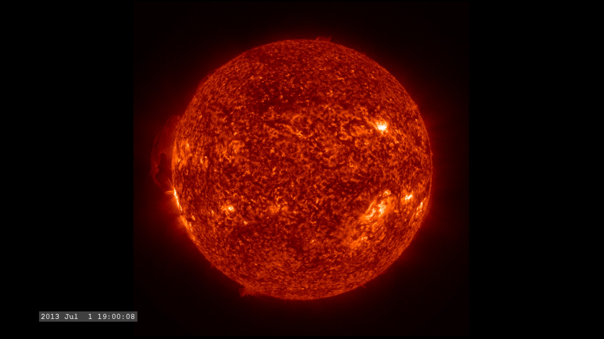
Solar Dynamics Observatory: April 21, 2015 Eruption on the Solar Limb
Go to this pageMovie of plasma eruption (upper left limb). || Apr2015LimbErupt_304A_stand.HD1080i.00945_print.jpg (1024x576) [73.9 KB] || Apr2015LimbErupt_304A_stand.HD1080i.00945_searchweb.png (320x180) [41.0 KB] || Apr2015LimbErupt_304A_stand.HD1080i.00945_thm.png (80x40) [3.5 KB] || Apr2015LimbErupt_304A_stand_1080p.webm (1920x1080) [6.4 MB] || 1920x1080_16x9_30p (1920x1080) [0 Item(s)] || Apr2015LimbErupt_304A_stand_1080p.mp4 (1920x1080) [43.2 MB] || Apr2015LimbErupt_304A_stand_1080p.mp4.hwshow [199 bytes] ||
2014
- ID: 4963
- ID: 4211
 Visualization
 - ID: 4232
 Visualization
 - ID: 4235
 Visualization
 - ID: 4228
 Visualization
 - ID: 11136
 Produced Video
 - ID: 4267
- ID: 11463
 Produced Video
 - ID: 4246
 Visualization
 - ID: 4244
- ID: 4065
 Visualization
 - ID: 4225
 Visualization
 - ID: 4216
 Visualization
 - ID: 4202
 Visualization
 - ID: 4166
 Visualization
 - ID: 4125
 Visualization
 - ID: 4182
 Visualization
 - ID: 4164
- ID: 11564
 Produced Video
 - ID: 11651
 Produced Video
 - ID: 11670
 Produced Video
 - ID: 4907
 Visualization
 - ID: 11721
 Produced Video
2013
- ID: 4031
 Visualization
 - ID: 11201
 Produced Video
 - ID: 4090
 Visualization
 - ID: 11379
 Produced Video
 - ID: 4089
 Visualization
 - ID: 4066
 Visualization
 - ID: 4051
 Visualization
 - ID: 4136
 Visualization
 - ID: 4133
 Visualization
 - ID: 10785
- ID: 11285
 Produced Video
 - ID: 4121
 Visualization
 - ID: 11298
 Produced Video
 - ID: 4101
 Visualization
 - ID: 11387
 Produced Video
2012
- ID: 4909
 Visualization
 - ID: 3999
 Visualization
 - ID: 11095
 Produced Video
 - ID: 4026
 Visualization
 - ID: 4761Visualization
- ID: 4038
 Visualization
 - ID: 11044
 Produced Video
 - ID: 4259
 Visualization
 - ID: 3919
 Visualization
 - ID: 4027
 Visualization
 - ID: 3920
- ID: 4034
 Visualization
 - ID: 4033

- ID: 4037
 Visualization
 - ID: 4150
 Visualization
 - ID: 3946
 Visualization
 - ID: 4309
 Visualization
 - ID: 3941
 Visualization
 - ID: 3940
 Visualization
 - ID: 11034
 Produced Video
 - ID: 3963
 Visualization
 - ID: 3922
 Visualization
2011
- ID: 3955
 Visualization
 - ID: 3945
 Visualization
 - ID: 4128
 Visualization
 - ID: 4117
 Visualization
 - ID: 4049
 Visualization
 - ID: 4151
 Visualization
 - ID: 3897
 Visualization
 - ID: 4352
- ID: 3838
- ID: 3839
- ID: 3840
- ID: 4250
 Visualization
 - ID: 3841
- ID: 3828
- ID: 3933
 Visualization
 - ID: 3932
 Visualization
 - ID: 3931
 Visualization
 - ID: 3929
 Visualization
 - ID: 3924
 Visualization
 - ID: 3923
 Visualization
 - ID: 4277
- ID: 3957
 Visualization
 - ID: 3978
 Visualization
 - ID: 3979
 Visualization
 - ID: 3980
 Visualization
 - ID: 3981
 Visualization
 - ID: 3982
 Visualization
 - ID: 3983
 Visualization
 - ID: 3984
 Visualization
 - ID: 3985
 Visualization
 - ID: 3986
 Visualization
 - ID: 3987
 Visualization
 - ID: 3989
 Visualization
 - ID: 3990
 Visualization
 - ID: 3988
 Visualization
2010
- ID: 3965 Visualization
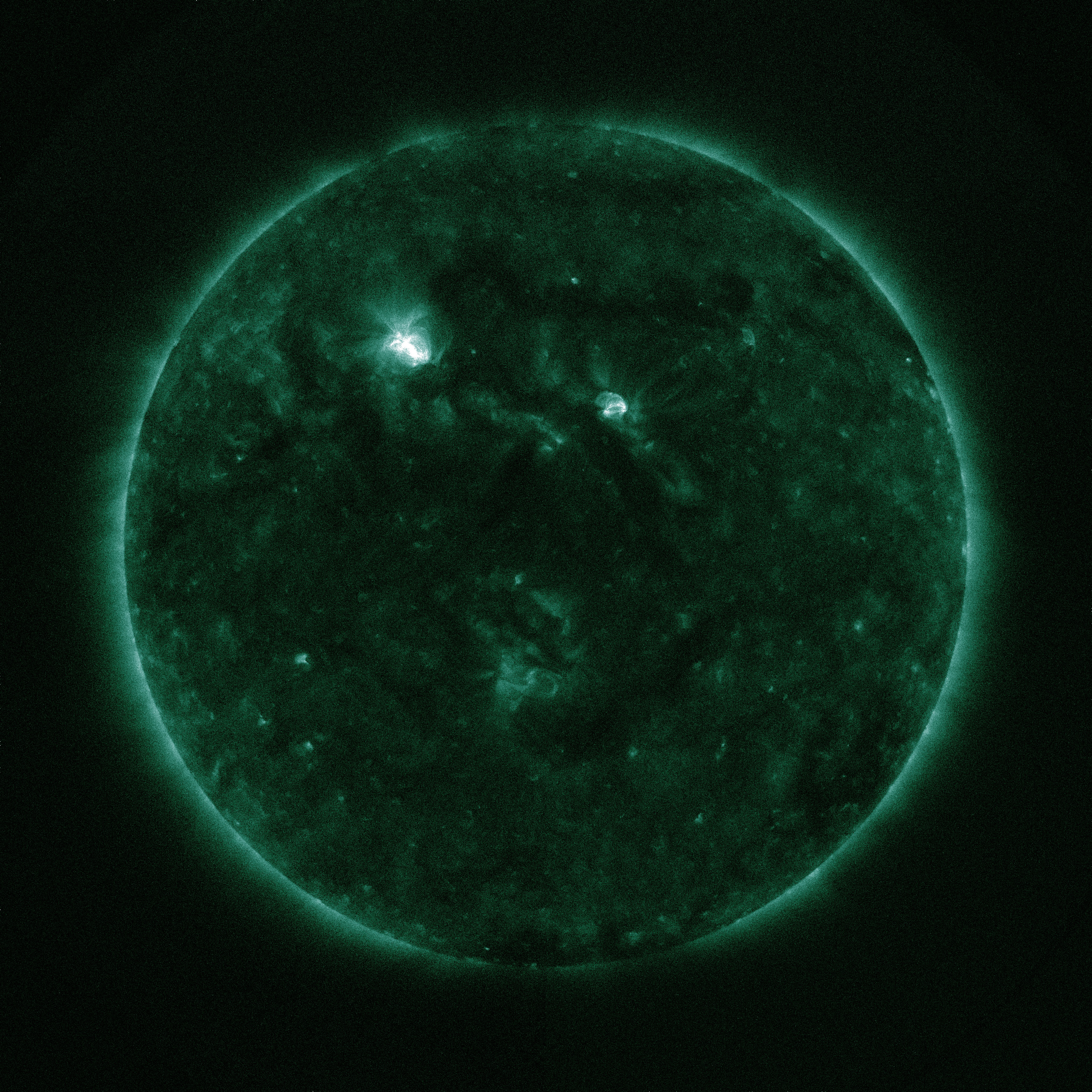
Impressionist Sun: SDO Source Images
Go to this pageA set of multi-wavelength views of the Sun from SDO provided source and context imagery for the Van Gogh Sun video. This video illustrates how imagery is converted into physical parameters teaching us more about the physical processes taking place in the solar atmosphere. ||
- ID: 4075 Visualization
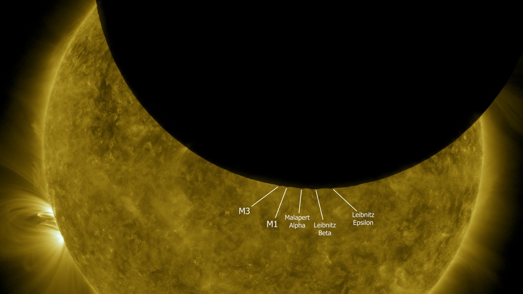
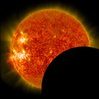
Lunar Transit from Solar Dynamics Observatory (2010)
Go to this pageJust as we do on Earth, the Solar Dynamics Observatory satellite periodically crosses the Moon's shadow and experiences a solar eclipse. During the eclipse witnessed by SDO on October 7, 2010, the southern hemisphere of the Moon was silhouetted against the solar disk, revealing some especially prominent mountain peaks near the Moon's south pole. By using elevation data from Lunar Reconnaissance Orbiter to visualize the Moon from SDO's point of view, it's possible to identify these peaks. Although all of these are well-known features, all but one of them have no official names. The following list corresponds to the labels in the animation, from left to right.In his 1954 sketch of the lunar south pole, astronomer Ewen Whitaker labeled this feature "M3." It's a mountain about halfway between the craters Cabeus and Drygalski, at 83.2°S 68°W.Whitaker's "M1," a mountain on the northern rim of Cabeus, 83.4°S 33°W.A mountain on the southern rim of Malapert crater, about halfway between the centers of Malapert and Haworth. Whitaker labels this Malapert Alpha. It's also known as Mons Malapert or Malapert Peak. 85.8°S 0°E.Labeled Leibnitz Beta by Whitaker and now officially named Mons Mouton, this is part of the highlands adjacent to the northern rim of Nobile crater. 84°S 37°E. Part of the Leibnitz mountain range first identified by Johann Schröter in the late 1700s, unrelated to Leibnitz Crater on the lunar far side.A mountain near Amundsen crater, on the western (Earthward) rim of Hédervári crater, 82.2°S 75°E. Whitaker tentatively labels this Leibnitz Epsilon in his sketch.The Moon visualization uses the latest albedo and elevation maps from Lunar Reconnaissance Orbiter (LRO). ||