Climate Essentials
Overview
This Climate Essentials multimedia gallery brings together the latest and most popular climate-related images, data visualizations and video features from Goddard Space Flight Center. For more multimedia resources on climate and other topics, search the Scientific Visualization Studio. To learn more about NASA's contribution to understanding Earth's climate, visit the Global Climate Change site.
Temperature Visualizations
- ID: 5450 Visualization
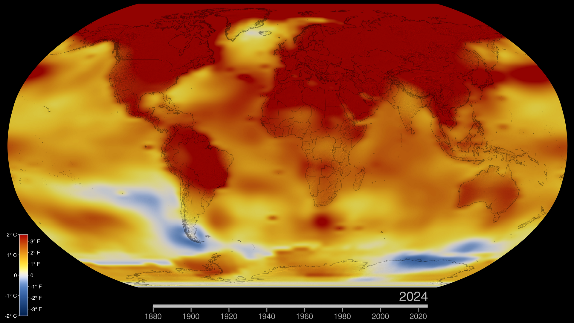
Global Temperature Anomalies from 1880 to 2024
Go to this pageThis color-coded map in Robinson projection displays a progression of changing global surface temperature anomalies. Normal temperatures are shown in white. Higher than normal temperatures are shown in red and lower than normal temperatures are shown in blue. Normal temperatures are calculated over the 30 year baseline period 1951-1980. The maps are averages over a running 24 month window. The final frame represents global temperature anomalies in 2024.
- ID: 5190 Visualization
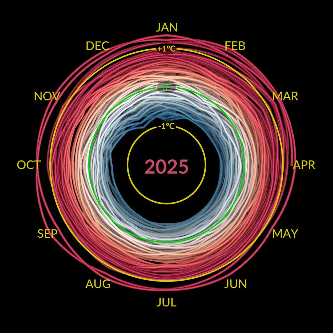
NASA Climate Spiral 1880-Present
Go to this pageThe NASA climate spiral visualization of the GISTEMP global temperature record.
- ID: 5376 Visualization
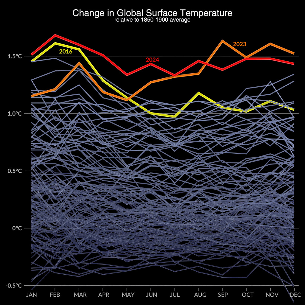
Record Temperature Years: 2024, 2023, and 2016
Go to this pageA visualization of global temperature anomalies highlighting the record years of 2024, 2023, and 2016. The visualizations morphs between a data grid showing monthly temperatures and a bar chart of annual temperatures. This version is labeled in English and temperatures are in Celsius. || GISTEMP_Records_English_C.00001_print.jpg (1024x1024) [402.0 KB] || GISTEMP_Records_English_C.00001_searchweb.png (320x180) [105.1 KB] || GISTEMP_Records_English_C.00001_thm.png [7.1 KB] || GISTEMP_Records_English_C.mp4 (2160x2160) [19.3 MB] || climate_compiled_GISTEMP.hwshow ||
- ID: 5451 Visualization
Zonal Climate Anomalies 1880-2024
Go to this pageA visualization of zonal temperature anomalies. The latitude zones are 90N-64N, 64N-44N, 44N-24N, 24N-EQU, EQU-24S, 24S-44S, 44S-64S, 64S-90S. The anomalies are calculated relative to a baseline period of 1951-1980. This version is in Celsius, an alternate version in Fahrenheit is also available. || GISTEMP_Zonal_1880-2024_C_2160p30.00850_print.jpg (1024x576) [52.4 KB] || GISTEMP_Zonal_1880-2024_C_2160p30.00850_searchweb.png (320x180) [17.8 KB] || GISTEMP_Zonal_1880-2024_C_2160p30.00850_thm.png [2.4 KB] || GISTEMP_Zonal_1880-2024_C_2160p30.mp4 (3840x2160) [20.3 MB] ||
- ID: 5452 Visualization
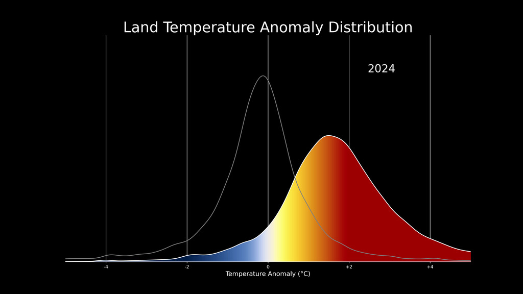
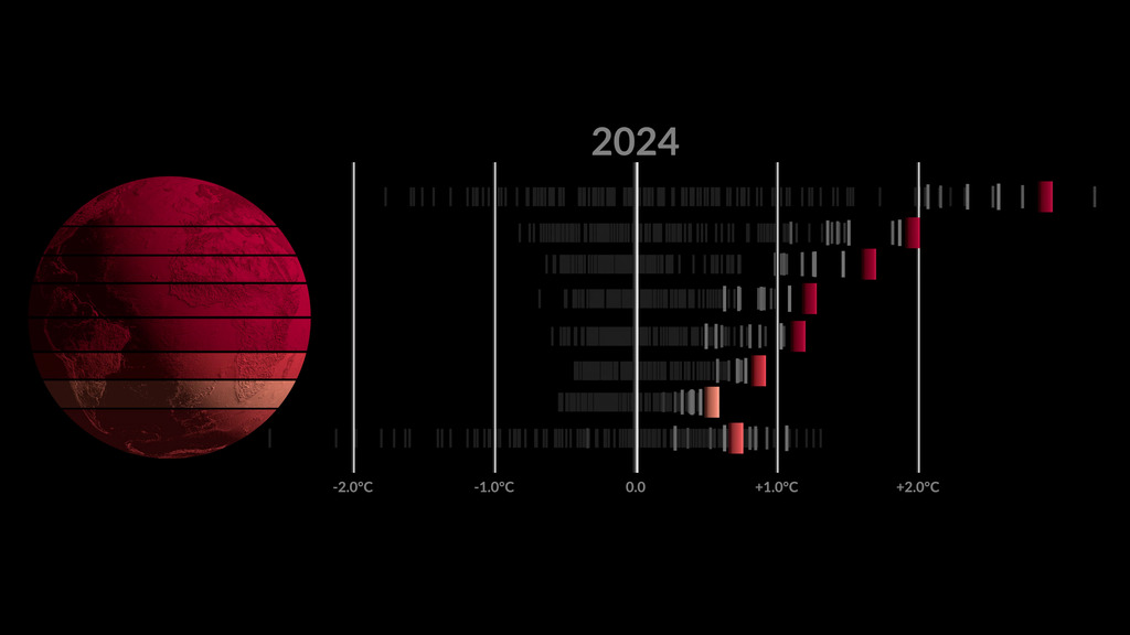
Shifting Distribution of Land Temperature Anomalies, 1964-2024
Go to this pageThe change in the distribution of land temperature anomalies over the years 1964 to 2024. This version is in Celsius, a Fahrenheit version is also available. || GISTEMPDist_2024_C.00850_print.jpg (1024x576) [45.7 KB] || GISTEMPDist_2024_C.00850_searchweb.png (320x180) [13.7 KB] || GISTEMPDist_2024_C.00850_thm.png [2.1 KB] || GISTEMPDist_2024_C.mp4 (3840x2160) [21.1 MB] ||
- ID: 4908 Visualization
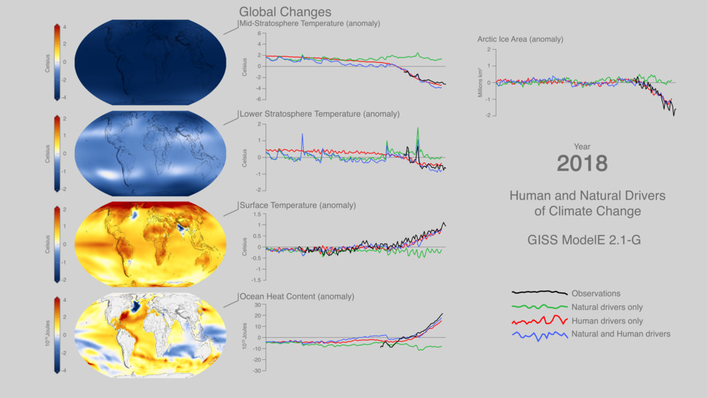
Climate Drivers
Go to this pageData visualization of human and natural drivers of climate change for the period 1850-2018, showcasing data products from NASA's GISS Model E 2.1-G and observations.Dr. Gavin Schmidt uses this visual to explain NASA's role in tracking and predicting climate at the 2021 COP26 conference - https://www.youtube.com/watch?v=CCAcKuJaJOg. || ClimateDrivers_3840x2160_30fps_923_print.jpg (1024x576) [106.7 KB] || ClimateDrivers_3840x2160_30fps_923_searchweb.png (320x180) [44.7 KB] || ClimateDrivers_3840x2160_30fps_923_thm.png (80x40) [4.9 KB] || ClimateDrivers_1080p30.mp4 (1920x1080) [13.2 MB] || ClimateDrivers_1080p30.webm (1920x1080) [3.6 MB] || Composite (3840x2160) [0 Item(s)] || ClimateDrivers_3840x2160p30.mp4 (3840x2160) [36.1 MB] || ClimateDrivers_3840x2160_30fps_923.tif (3840x2160) [31.7 MB] || ClimateDrivers_1080p30.mp4.hwshow ||
Sea Level Change Visualizations
- ID: 5235 Visualization
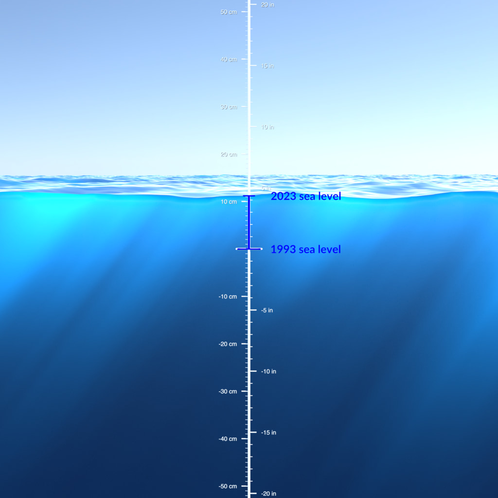
Sea Level Through a Porthole (2023)
Go to this pageAs the planet warms and polar ice melts, our global average sea level is rising. Although exact ocean heights vary due to local geography, climate over time, and dynamic fluid interactions with gravity and planetary rotation, scientists observe sea level trends by comparing measurements against a 20 year spatial and temporal mean reference. These visualizations use the visual metaphor of a submerged porthole window to observe how far our oceans rose between 1993 and 2023. ||
- ID: 5221 Visualization
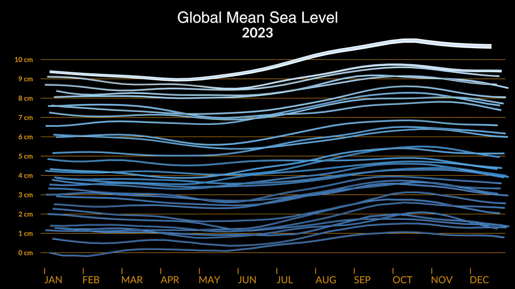
Global Mean Sea Level 1993-2023
Go to this pageThis animation shows the rise in global mean sea level from 1993 to 2023 based on data from a series of five international satellites. The spike in sea level from 2022 to 2023 is mostly a consequence of climate change and the development of El Niño conditions in the Pacific Ocean. || seaLevelRise_2024_English.00405_print.jpg (1024x576) [188.5 KB] || seaLevelRise_2024_English.00405_web.png (320x180) [54.4 KB] || seaLevelRise_2024_English.00405_thm.png (80x40) [5.1 KB] || seaLevel_Curves_2024_English.00405_searchweb.png (320x180) [41.9 KB] || English (3840x2160) [0 Item(s)] || seaLevelRise_2024_English.mp4 (3840x2160) [45.0 MB] || Climate-dashboard.hwshow [1.6 KB] ||
Greenhouse Gas Visualizations
- ID: 5196
 Visualization
 - ID: 5110
 Visualization
 - ID: 5447
 Visualization
 - ID: 4799
 Visualization
 - ID: 4962
- ID: 4908Visualization
- ID: 5041
 Visualization
 - ID: 5007
 Visualization
 - ID: 30556
 Hyperwall Visual
 - ID: 5054
 Visualization
 - ID: 5024
- ID: 5360
 Visualization
 - ID: 5332
 Visualization
 - ID: 5389
 Visualization
 - ID: 5272
 Visualization
 - ID: 5116
 Visualization
 - ID: 5115
 Visualization
Visualizations
- ID: 4974
 Visualization
 - ID: 5030
 Visualization
 - ID: 5036
 Visualization
 - ID: 5028
 Visualization
 - ID: 31156
 Visualization
 - ID: 31158
 Visualization
 - ID: 31166
 Visualization
 - ID: 4949
 Visualization
 - ID: 4914
 Visualization
 - ID: 4925
 Visualization
 - ID: 13557
- ID: 4935
 Visualization
 - ID: 4727
- ID: 4972
 Visualization
 - ID: 4834
Produced Pieces
- ID: 14066 Produced Video
![Universal Production Music: Knock and Wait (Instrumental) by Brice Davoli [SACEM], Well That’s Difference (Instrumental) by Jeff Cardoni [ASCAP], Wanna Be Hipster (Instrumental) by Jeff Cardoni [ASCAP], Curiosity Killed Kitty (Instrumental) by Robert Leslie Bennett [ASCAP], Eco Issues (Instrumental) by Max van Thun [GEMA] Additional Footage: Pond5.com, CSPANComplete transcript available.](/vis/a010000/a014000/a014066/Title.jpg)
Temperature Record 101: How We Know What We Know
Go to this page2021 was tied for the sixth warmest year on NASA’s record, stretching more than a century. But, what is a temperature record?GISTEMP, NASA’s global temperature analysis, takes in millions of observations from instruments on weather stations, ships and ocean buoys, and Antarctic research stations, to determine how much warmer or cooler Earth is on average from year to year.Stretching back to 1880, NASA’s record shows a clear warming trend. However, individual weather events and La Niña — a pattern of cooler waters in the Pacific that was responsible for slightly cooling 2021’s average temperature — can affect individual years.Because the record is global, not every place on Earth experienced the sixth warmest year on record. Some places had record-high temperatures, and we saw record droughts, floods and fires around the globe. ||
- ID: 13979 Produced Video
![Music: Futurity by Lee Groves [PRS] and Peter George Marett [PRS]Complete transcript available.](/vis/a010000/a013900/a013979/Screen_Shot_2021-10-28_at_2.29.18_PM.png)
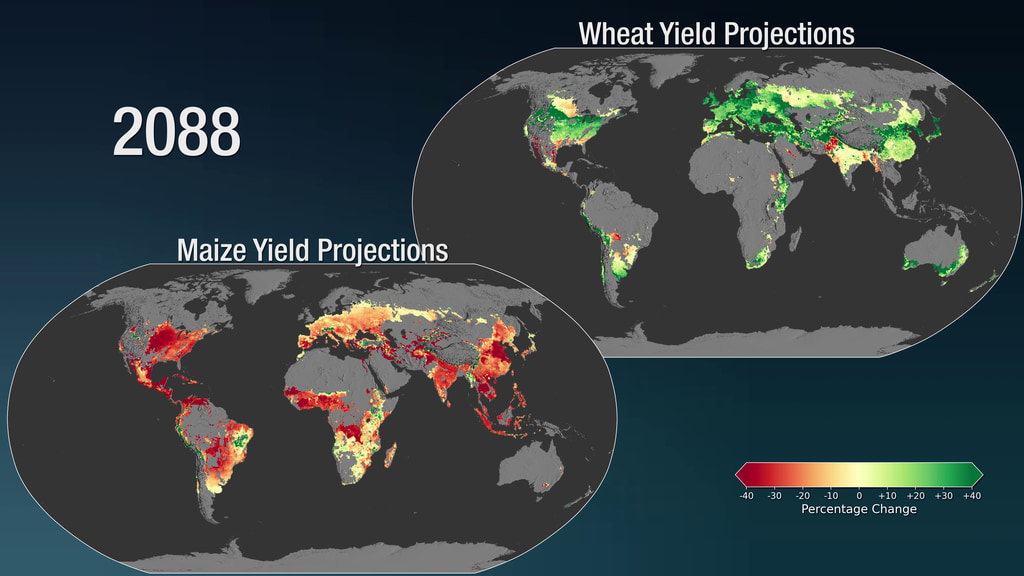
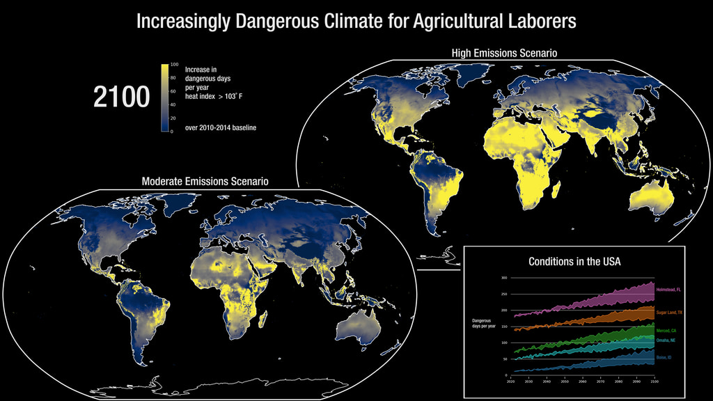
Climate Change Could Affect Global Agriculture within 10 Years
Go to this pageAverage global crop yields for maize, or corn, may see a decrease of 24% by late century, with the declines becoming apparent by 2030, with high greenhouse gas emissions, according to a new NASA study. Wheat, in contrast, may see an uptick in crop yields by about 17%. The change in yields is due to the projected increases in temperature, shifts in rainfall patterns and elevated surface carbon dioxide concentrations due to human-caused greenhouse gas emissions, making it more difficult to grow maize in the tropics and expanding wheat’s growing range. ||
- ID: 13839 Produced Video
![Music: Dawn Drone by Juan Jose Alba Gomez [SGAE]Complete transcript available.](/vis/a010000/a013800/a013839/Thumbnail_print.jpg)
Warmer Ocean Temperatures May Decrease Saharan Dust Crossing the Atlantic
Go to this pageEvery year millions of tons of dust from the Sahara Desert are swirled up into the atmosphere by easterly trade winds, and carried across the Atlantic. The plumes can make their way from the African continent as far as the Amazon rainforest, where they fertilize plant life.As the climate changes, dust activity will continue to be affected. In a new study, NASA researchers predict that within the next century we will see dust transport approach a 20,000-year minimum. ||
- ID: 13699 Produced Video
![Music: "Dew" by Matthew Nicholson [PRS], Suki Jeanette Finn [PRS]This video can be freely shared and downloaded. While the video in its entirety can be shared without permission, some individual imagery provided by pond5.com is obtained through permission and may not be excised or remixed in other products. Specific details on stock footage may be found here. For more information on NASA’s media guidelines, visit https://www.nasa.gov/multimedia/guidelines/index.html.Complete transcript available.](/vis/a010000/a013600/a013699/ImjaLake.jpg)
Tracking Three Decades of Dramatic Glacial Lake Growth
Go to this pageMusic: "Dew" by Matthew Nicholson [PRS], Suki Jeanette Finn [PRS]This video can be freely shared and downloaded. While the video in its entirety can be shared without permission, some individual imagery provided by pond5.com is obtained through permission and may not be excised or remixed in other products. Specific details on stock footage may be found here. For more information on NASA’s media guidelines, visit https://www.nasa.gov/multimedia/guidelines/index.html.Complete transcript available. || ImjaLake.jpg (1920x1080) [1.2 MB] || ImjaLake_print.jpg (1024x576) [382.8 KB] || ImjaLake_searchweb.png (320x180) [109.6 KB] || ImjaLake_web.png (320x180) [109.6 KB] || ImjaLake_thm.png (80x40) [7.5 KB] || 13699_GlacierLake820.mov (1920x1080) [1.9 GB] || 13699_GlacierLake820.mp4 (1920x1080) [138.4 MB] || 13699_GlacierLake820.webm (1920x1080) [15.0 MB] || GlacierLake820.en_US.srt [2.1 KB] || GlacierLake820.en_US.vtt [2.1 KB] ||
- ID: 13781 Produced Video
![Music: A Curious Incident by Jay Price [PRS] and Paul Reeves [PRS]Complete transcript available.](/vis/a010000/a013700/a013781/CO20.jpg)
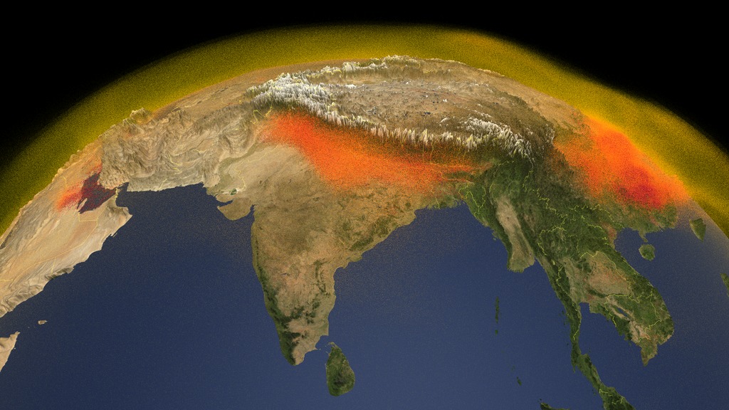
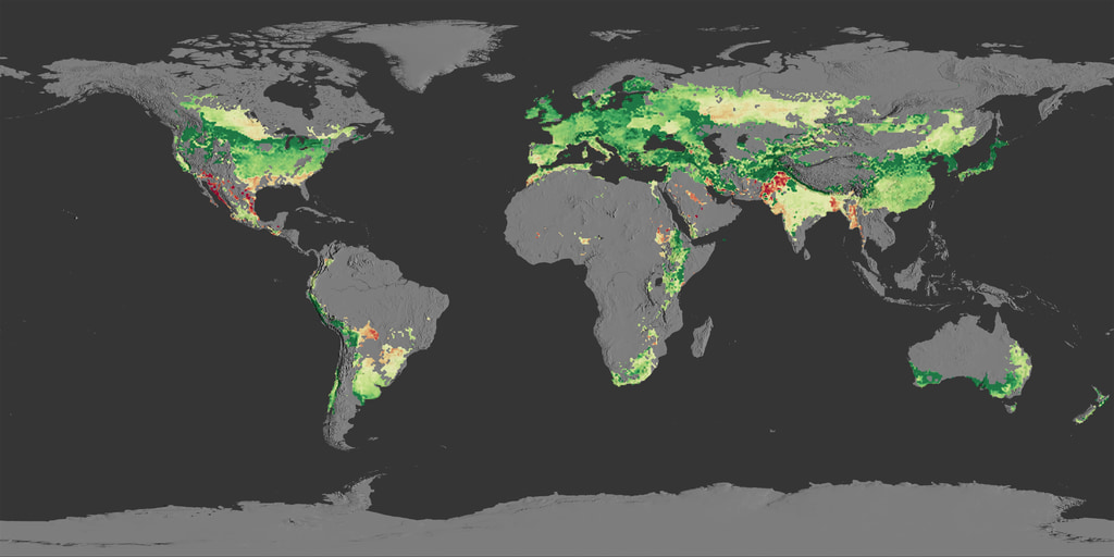
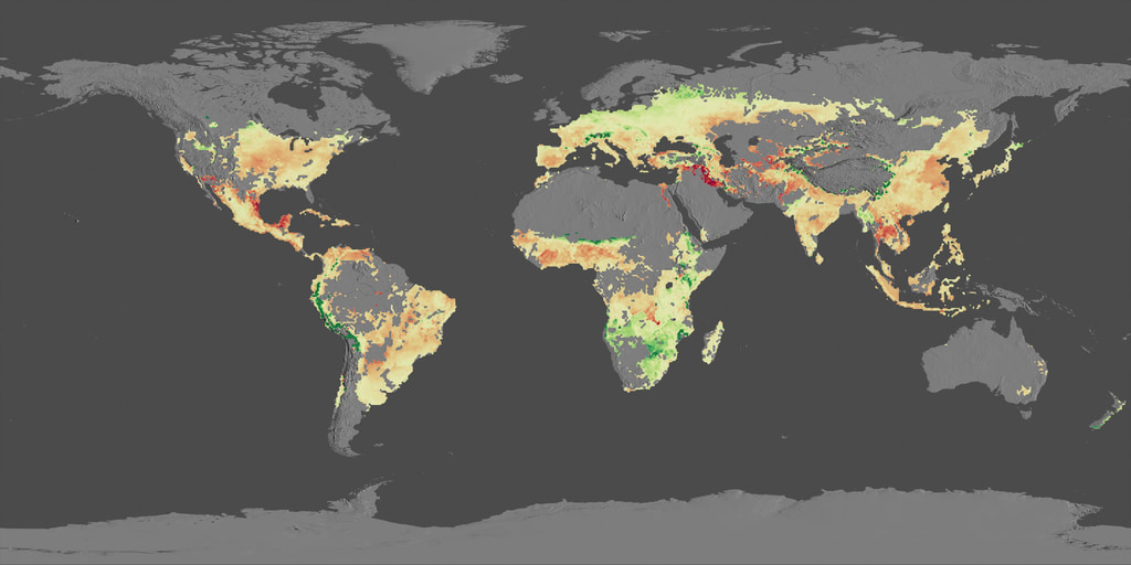
Plants Are Struggling to Keep Up with Rising Carbon Dioxide Concentrations
Go to this pagePlants play a key role in mitigating climate change. The more carbon dioxide they absorb during photosynthesis, the less carbon dioxide remains trapped in the atmosphere where it can cause temperatures to rise. But scientists have identified an unsettling trend – 86% of land ecosystems globally are becoming progressively less efficient at absorbing the increasing levels of CO2 from the atmosphere. ||
- ID: 13559 Produced Video
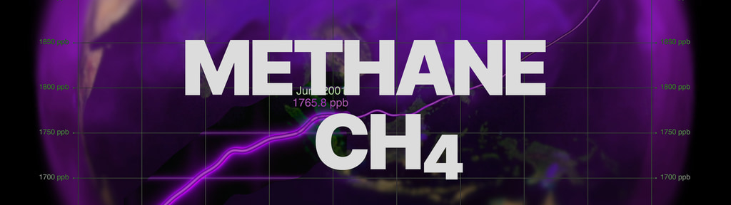
![Complete transcript available.Music: "Reported Missing" by Andrew Michael Britton [PRS] and David Stephen Goldsmith [PRS]This video can be freely shared and downloaded. While the video in its entirety can be shared without permission, some individual imagery provided by Artbeats is obtained through permission and may not be excised or remixed in other products. Specific details on stock footage may be found here. For more information on NASA’s media guidelines, visit https://www.nasa.gov/multimedia/guidelines/index.html.](/vis/a010000/a013500/a013559/Methane_Still.jpg)
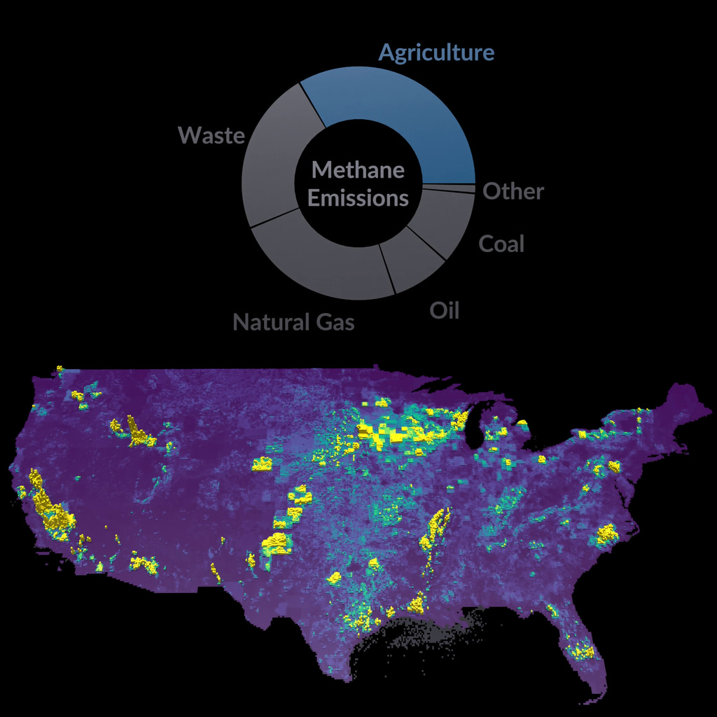
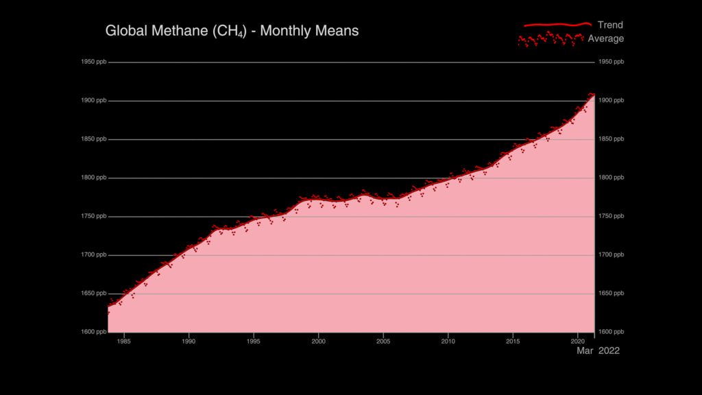
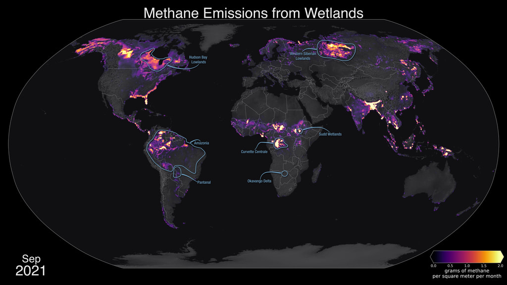
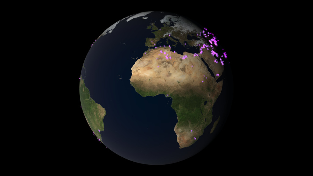
NASA Models Methane Sources and Movement Around the Globe
Go to this pageComplete transcript available.Music: "Reported Missing" by Andrew Michael Britton [PRS] and David Stephen Goldsmith [PRS]This video can be freely shared and downloaded. While the video in its entirety can be shared without permission, some individual imagery provided by Artbeats is obtained through permission and may not be excised or remixed in other products. Specific details on stock footage may be found here. For more information on NASA’s media guidelines, visit https://www.nasa.gov/multimedia/guidelines/index.html. || Methane_Still.jpg (1920x1080) [408.5 KB] || Methane_Still_print.jpg (1024x576) [181.8 KB] || Methane_Still_searchweb.png (180x320) [71.4 KB] || Methane_Still_web.png (320x180) [71.4 KB] || Methane_Still_thm.png (80x40) [6.4 KB] || 13559_Methane_Final.webm (960x540) [62.2 MB] || TWITTER_720_13559_Methane_Final_twitter_720.mp4 (1280x720) [28.5 MB] || 13559_Methane_Final_lowres.mp4 (1280x720) [43.6 MB] || 13559_Methane_Final.mp4 (1920x1080) [272.5 MB] || Mathen_captions.en_US.srt [3.2 KB] || Mathen_captions.en_US.vtt [3.3 KB] || 13559_Methane_Final.mov (1920x1080) [3.4 GB] ||
- ID: 13799 Produced Video
![Music: Organic Machine by Bernhard Hering [GEMA] and Matthias Kruger [GEMA]Complete transcript available.](/vis/a010000/a013700/a013799/2020Temp.png)
NASA Finds 2020 Tied for Hottest Year on Record
Go to this pageGlobally, 2020 was the hottest year on record, effectively tying 2016, the previous record. Overall, Earth’s average temperature has risen more than 2 degrees Fahrenheit since the 1880s. Temperatures are increasing due to human activities, specifically emissions of greenhouse gases, like carbon dioxide and methane. ||
- ID: 13233 Produced Video
![Music: Tides by Jon Cotton [PRS], Ben Niblett [PRS]Complete transcript available.](/vis/a010000/a013200/a013233/Greenland_Still_Two.jpg)
Modeling the Future of the Greenland Ice Sheet
Go to this pageMusic: Tides by Jon Cotton [PRS], Ben Niblett [PRS]Complete transcript available. || Greenland_Still_Two.jpg (1920x1080) [941.0 KB] || Greenland_Still_Two_searchweb.png (320x180) [152.3 KB] || Greenland_Still_Two_thm.png (80x40) [8.8 KB] || 13233_Greenland_Outlet_FINAL.mp4 (1920x1080) [253.2 MB] || 13233_Greenland_Outlet_FINAL.mov (1920x1080) [3.4 GB] || 13233_Greenland_Outlet_FINAL.webm (1920x1080) [17.2 MB] || 13233_Greenland_Outlet_FINAL_VX-303985.webm (960x540) [54.0 MB] || GreenlandOutletModel_Fine_V2.en_US.srt [2.9 KB] || GreenlandOutletModel_Fine_V2.en_US.vtt [2.9 KB] ||
- ID: 14631 Produced Video
![Universal Production Music: Prismatic by David Stephen Goldsmith [ PRS ]Complete transcript available.](/vis/a010000/a014600/a014631/14631_DYAMONDThumbnailHorz.jpg)
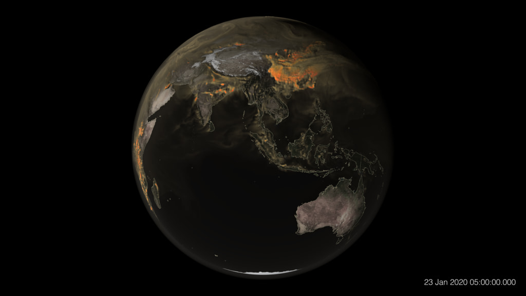
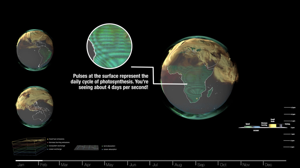
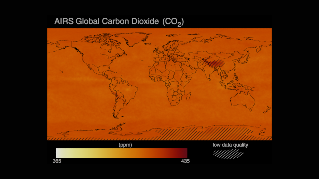
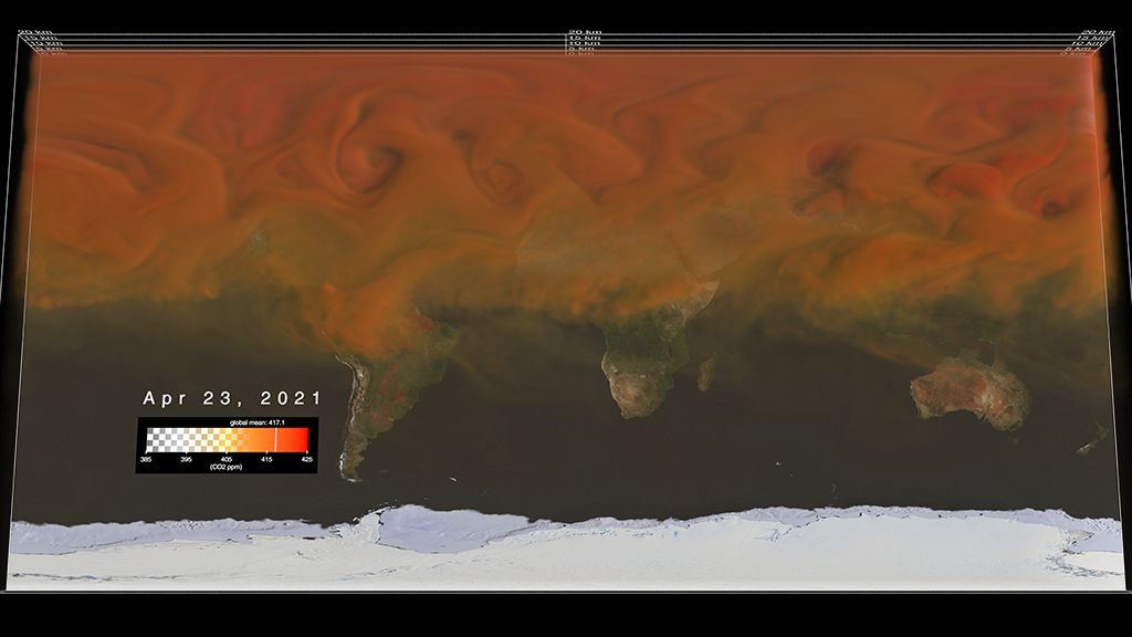
Model Behavior: Visualizing Global CO2
Go to this pageUniversal Production Music: Prismatic by David Stephen Goldsmith [ PRS ]Complete transcript available. || 14631_DYAMONDThumbnailHorz.jpg (1280x720) [291.1 KB] || 14631_DYAMONDThumbnailHorz_print.jpg (1024x576) [222.2 KB] || 14631_DYAMONDThumbnailHorz_searchweb.png (320x180) [91.4 KB] || 14631_DYAMONDThumbnailHorz_thm.png (80x40) [7.1 KB] || 14631_dyamondhorz_US.en.en_US.srt [2.3 KB] || 14631_dyamondhorz_US.en.en_US.vtt [2.2 KB] || 14631_DYAMOND_Horz.webm (3840x2160) [32.4 MB] || 14631_DYAMOND_Horz.mp4 (3840x2160) [267.6 MB] ||
- ID: 14568 Produced Video
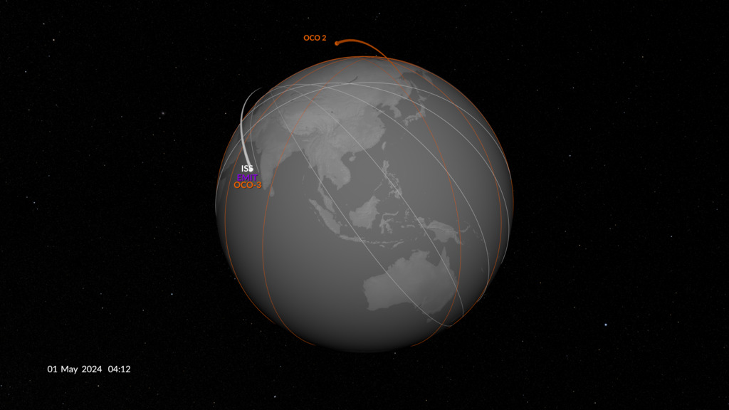
Tracking the Greenhouse Gas Methane, Earth Information Center Videos
Go to this pageFull 8K resolution. Optimized for Earth Information Center display.Universal Production Music: "Passing By" by Miguel D'Oliveira, "Simple Story" by Fred Dubois, and "Whispers of Hope" by Sam Connelly, This video can be freely shared and downloaded. While the video in its entirety can be shared without permission, some individual imagery provided by Pond5 and The Raleigh Drone Company is obtained through permission and may not be excised or remixed in other products. For more information on NASA’s media guidelines, visit https://www.nasa.gov/multimedia/guidelines/index.html || GHGMain.png (7680x2160) [5.4 MB] || GHGMain_print.jpg (1024x288) [68.0 KB] || GHGMain_searchweb.png (320x180) [64.0 KB] || GHGMain_thm.png (80x40) [6.8 KB] || GHG.en_US.srt [4.0 KB] || GHG.en_US.vtt [3.8 KB] || GHG_Main_7680x2160.mp4 (7680x2160) [586.6 MB] || GHG_Main.mp4 (7680x2160) [1.1 GB] || GHG_Main_h.264.mov (7680x2160) [1.1 GB] ||
Animations
- ID: 20328 Animation
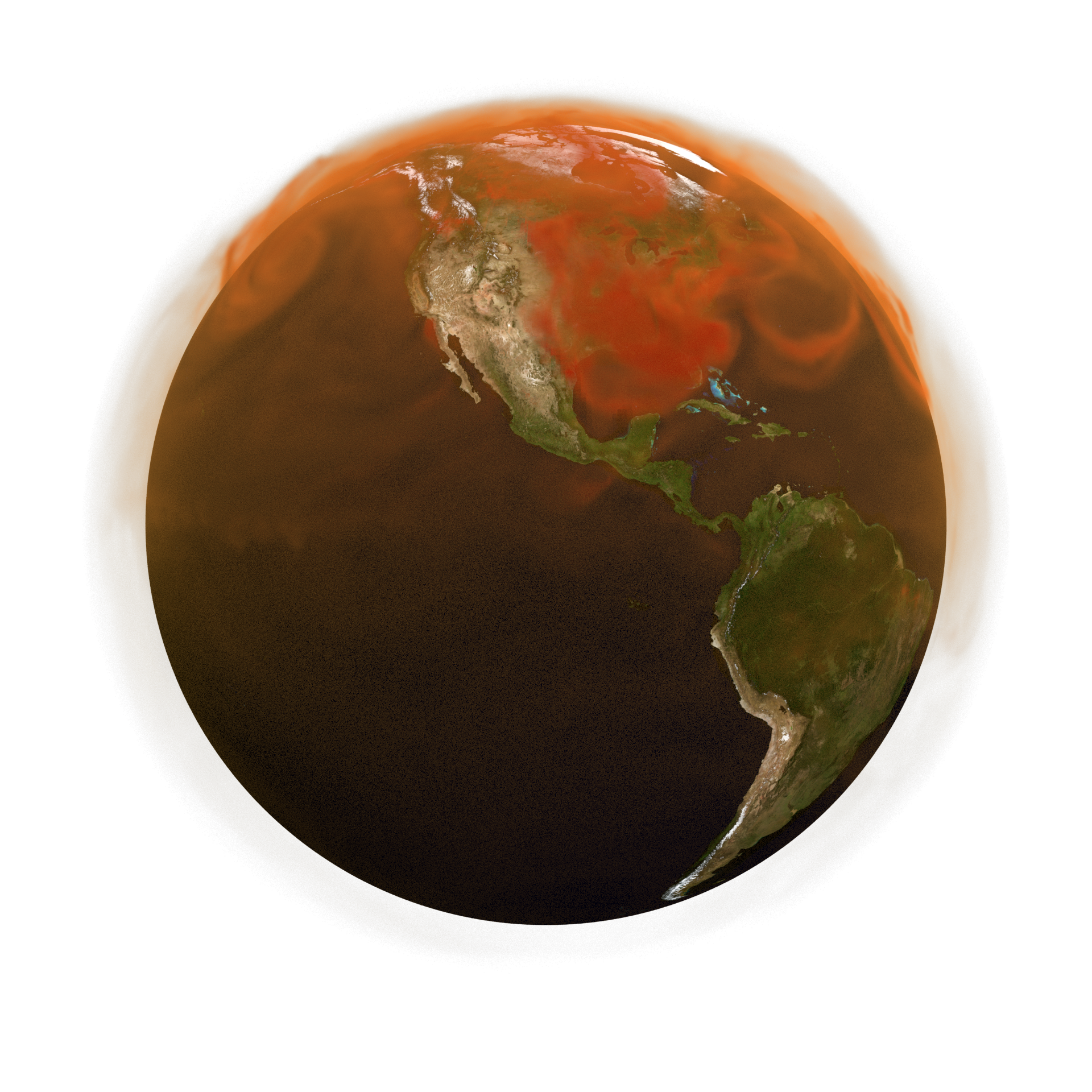
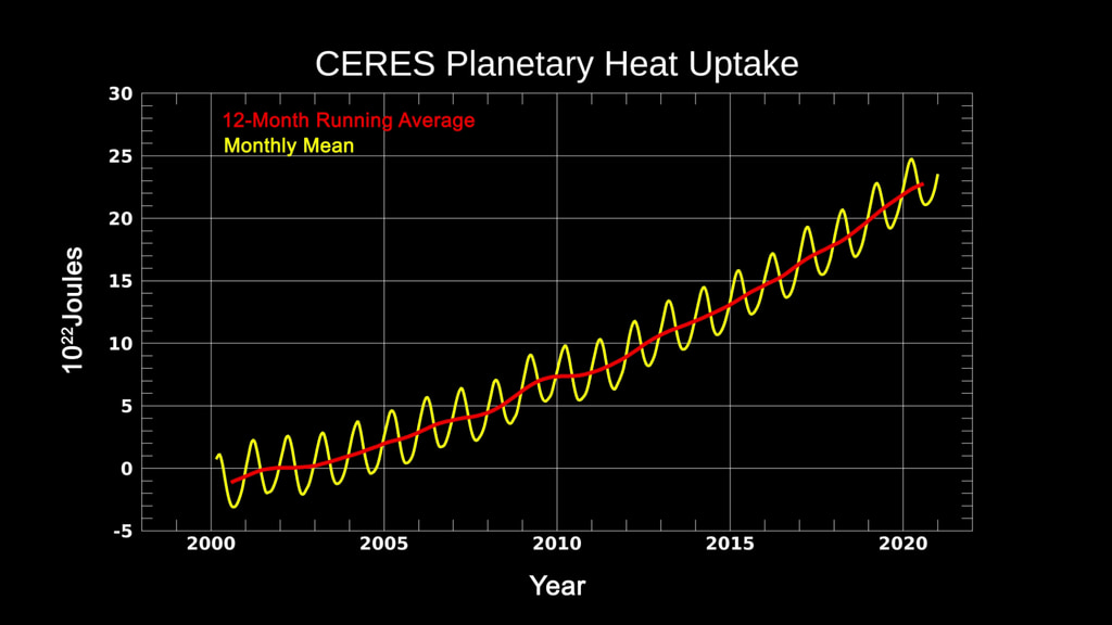
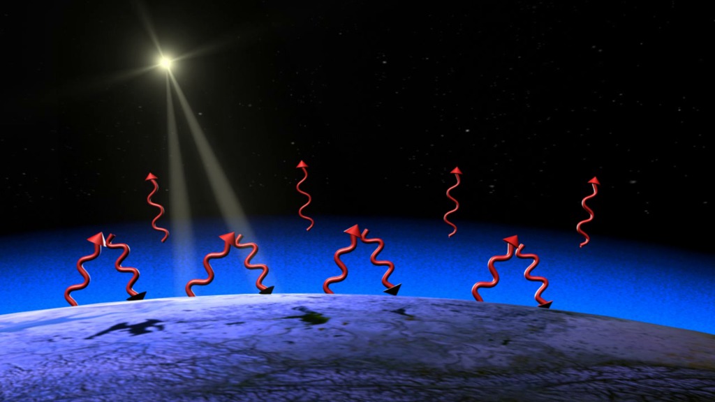
Radiative Forcing
Go to this pageA simplified animation of Earth's planetary energy balance: A planet’s energy budget is balanced between incoming (yellow) and outgoing radiation (red); On Earth, natural and human-caused processes affect the amount of energy received as well as emitted back to space; This study filters out variations in Earth’s energy budget due to feedback processes, revealing the energy changes caused by aerosols and greenhouse gas emissions. ||
- ID: 20114 Animation
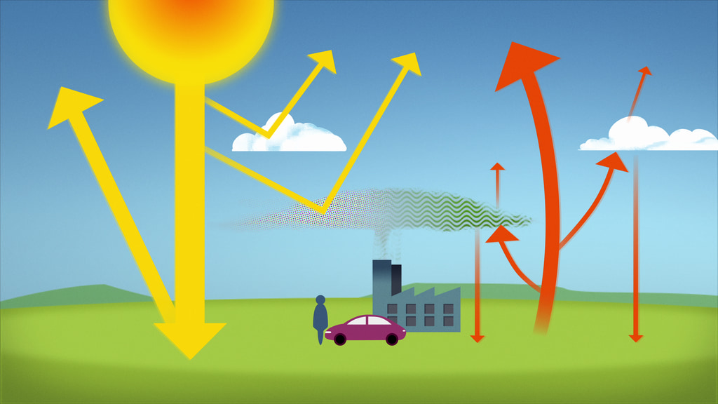
Greenhouse Gases Effect on Global Warming
Go to this pageThe 'greenhouse effect' is the warming of climate that results when the atmosphere traps heat radiating from Earth toward space. Certain gases in the atmosphere resemble glass in a greenhouse, allowing sunlight to pass into the 'greenhouse,' but blocking Earth's heat from escaping into space. The gases that contribute to the greenhouse effect include water vapor, carbon dioxide (CO2), methane, nitrous oxides, and chlorofluorocarbons (CFCs).On Earth, human activities are changing the natural greenhouse. Over the last century the burning of fossil fuels like coal and oil has increased the concentration of atmospheric CO2. This happens because the coal or oil burning process combines carbon (C) with oxygen (O2) in the air to make CO2. To a lesser extent, the clearing of land for agriculture, industry, and other human activities have increased the concentrations of other greenhouse gases like methane (CH4), and further increased (CO2).The consequences of changing the natural atmospheric greenhouse are difficult to predict, but certain effects seem likely: - On average, Earth will become warmer. Some regions may welcome warmer temperatures, but others may not. - Warmer conditions will probably lead to more evaporation and precipitation overall, but individual regions will vary, some becoming wetter and others dryer. - A stronger greenhouse effect will probably warm the oceans and partially melt glaciers and other ice, increasing sea level. Ocean water also will expand if it warms, contributing to further sea level rise. - Meanwhile, some crops and other plants may respond favorably to increased atmospheric CO2, growing more vigorously and using water more efficiently. At the same time, higher temperatures and shifting climate patterns may change the areas where crops grow best and affect the makeup of natural plant communities. ||