|
4 THE PIPELINE Once the registration shader had been developed, the process for creating the zooms became clear. A first render pass using the images with the registration shader would determine whether the registration was adequate for feature matching between images. Follow-up passes could then be repeatedly rendered using the registration shader as the images were color matched to each other until the color differences were imperceptible.
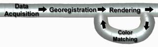
Figure 3: The Development Pipeline Two primary steps precede rendering and color matching. First, data must be acquired for each level, and then the data must be transformed into color imagery that is registered to geographic coordinates. These four processes (acquisition, georegistration, color matching, and rendering) will now be described in further detail. 4.1 Data Acquisition The first step in our pipeline is data acquisition. Having selected a zoom location, we needed to locate data at the various resolutions. There were several considerations when identifying which data sets to use. Our first priority was to obtain cloud-free imagery. This can be particularly challenging in certain regions (e.g., Seattle) and at sizes covering large areas (e.g., 250-meter data sets covering the entire East Coast). Our second priority was to obtain data sets that were acquired as close as possible to each other in time or at least relative to the season. We reused the same 4-kilometer global data set from MODIS for most of the zooms. This presented some problems, primarily when creating zooms into northern cities where snow cover may have been different. The regional MODIS 250-meter data sets needed to be cloud free for about 1000 kilometers around the city. It proved to be challenging to find cloudless data sets covering this large an area for dates corresponding to the smaller scale data sets. The local 15-meter data sets from Landsat 7 tended to be the easiest data sets to acquire. Landsat scenes cover small enough areas that locating cloud-free data was less difficult. In addition, Landsat has a long history of data sets to draw from with a robust and efficient ordering system. Space Imaging's IKONOS satellite provided the 1-meter data sets. These data sets tended to be more difficult to acquire. Since the area of IKONOS coverage is so small (roughly 10 km by 10 km), there are fewer occasions when data can be taken for a particular area. In addition, IKONOS was a relatively new satellite with fewer archival data sets to draw from. A general problem that we had was finding data sets that were centered near our landmarks of interest. We needed to maintain the resolution in all directions to a certain point before transitioning to the next data set or blurring would result at the transition edges between data sets. |
4.2 Georegistration Each data set consists of a series of 8-bit or 16-bit gray scale images in instrument specific frequency bands and a panchromatic image at a higher spatial resolution. The 16-bit images were re-scaled to 8-bit since we did not need the higher color resolution, and 8-bit images can be manipulated with more image software. The panchromatic bands were used to sharpen the individual frequency channels to the higher resolution using Principal Component Substitution [9]. In some cases, this method would alter the color balance of the resulting RGB images, but this was not a serious issue since significant color alteration would still be necessary to match the images to each other. ERDAS Imagine was used to pan-sharpen IKONOS imagery to 1-meter resolution and Landsat imagery to 15-meter resolution. MODIS imagery was usually acquired at the pan-sharpened 250-meter resolution. Imagine was also used to transform the imagery from the Universal Transverse Mercator projection to geographic coordinate-aligned rectangles and to perform the registration adjustments to achieve feature-level matching between pairs of images. The ability of Imagine to load multiple images at the maximum texture resolution of RenderMan (16,384 x 16,384 pixels) and display the images with correct geospatial registration was invaluable. The output from this phase was the four registered images and the associated longitude/latitude extents of the images for use in the rendering phase. 4.3 Color Matching Color matching was the most time consuming and perhaps most important phase of our pipeline. Without extremely close color matching between data sets, our goal of a seamless zoom would be impossible due to the sensitivity of the human eye to variations in color. This phase was also unique in that it required artistic ability to complete the tasks. We used Photoshop to perform color matching. Our general approach was to first make the 1-meter IKONOS image look as realistic as possible, particularly around the chosen zoom location. We also created an alpha mask for each image (except for the global image) so that the registration shader could blend each image into the next layer. We next created a scaled-down version of the IKONOS image to overlay the Landsat 15-meter image in order to see how the Landsat color needed to be adjusted to match. Adjustment layers were our primary means of color matching [10]. We most often used Color Balance, Hue/Saturation, Levels, Curves, and Brightness/Contrast. A common test we used when we thought we had a seamless transition between images was to ask people not involved in the project if they could detect any seams in the image. We repeated this process with the MODIS 250-meter and MODIS 4-kilometer images. We often had problems once we reached the global 4-kilometer image in that colors were propagated up through the image layers causing regions or even the globe to appear unnatural in color. In these cases, we reworked the problem colors through all four layers. This process was slow, and it was exacerbated by the fact that image files were so large (about one gigabyte each). Simply saving and loading each file took about 30 minutes. Once a good candidate set of images for each data set was color matched, those images were passed to the next phase of the pipeline: Rendering. |