Hyperwall Earth
Overview
Hyperwall stories in the Earth Category
Return to Main Hyperwall Gallery.
New
- Section

- ID: 30699 Hyperwall Visual
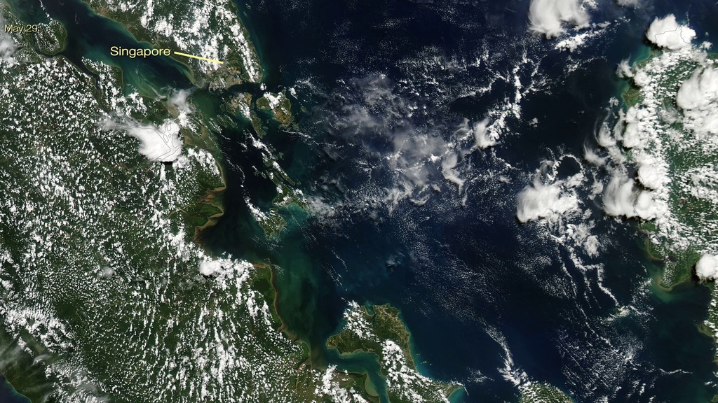
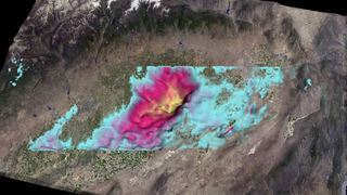
Hazardous Air Quality Conditions in Singapore
Go to this pageSingapore region on September 24 and May 25, 2015, MODIS data only || singapore_smog_24_1080p_print.jpg (1024x576) [279.3 KB] || singapore_smog_24_1080p_searchweb.png (180x320) [129.9 KB] || singapore_smog_24_1080p_thm.png (80x40) [8.0 KB] || singapore_smog_24_1080p.mp4 (1920x1080) [7.0 MB] || singapore_smog_24_720p.mp4 (1280x720) [3.8 MB] || singapore_smog_24_720p.webm (1280x720) [4.6 MB] || singapore_modis_only_24_2304p.mp4 (4096x2304) [20.4 MB] || singapore_smog_24_360p.mp4 (640x360) [1.2 MB] || singapore_smog_ver2a.key [8.5 MB] || singapore_smog_ver2a.pptx [5.8 MB] ||
- Section
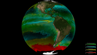
Ocean Surface CO2 Flux with Wind Stress
Go to this sectionThis animation shows the ocean surface CO2 flux between 1/1/2009 and 12/31/2010. Blue colors indicate uptake and orange-red colors indicate outgassing of ocean carbon. The pathlines indicate surface wind stress.
Beautiful Earth
Inspiring and classic scenes of Earth
- Section

Blue Marble 2002
Go to this sectionThis spectacular blue marble image was the most detailed true-color image of the entire Earth to date in 2002. Using a collection of satellite-based observations, scientists and visualizers stitched together months of observations of the land surface, oceans, sea ice, and clouds into a seamless, true-color mosaic of every square kilometer (.386 square mile) of our planet. The full resolution version of the image is 21,600 pixels across.
- Section
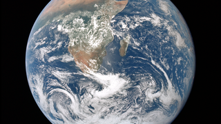
The Blue Marble From Apollo 17
Go to this sectionThis classic photograph of the Earth was taken on December 7, 1972. This is a version of the image prepared for use on the hyperwall. The original caption is reprinted below: View of the Earth as seen by the Apollo 17 crew traveling toward the moon. This translunar coast photograph extends from the Mediterranean Sea area to the Antarctica south polar ice cap. This is the first time the Apollo trajectory made it possible to photograph the south polar ice cap. Note the heavy cloud cover in the Southern Hemisphere. Almost the entire coastline of Africa is clearly visible. The Arabian Peninsula can be seen at the northeastern edge of Africa. The large island off the east coast of Africa is the Republic of Madagascar. The Asian mainland is on the horizon toward the northeast.
- ID: 30610 Hyperwall Visual
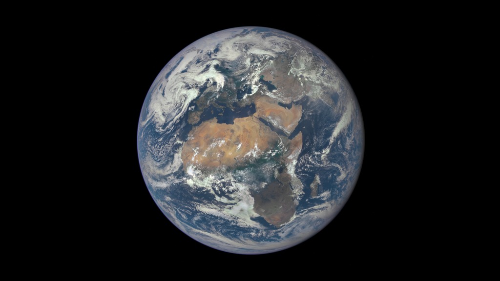
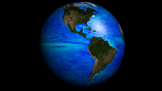
EPIC View of Earth
Go to this pageImages from DSCOVR have been prepared for use on the Hyperwall. On July 6, 2015, a NASA camera onboard the Deep Space Climate Observatory (DSCOVR) satellite returned its first view of the entire sunlit side of Earth from its orbit at the first Lagrange point (L1), about one million miles from Earth. This initial image, taken by DSCOVR’s Earth Polychromatic Imaging Camera (EPIC), shows the effects of sunlight scattered by air molecules, giving the image a characteristic bluish tint. Once the instrument begins regular data acquisition, images will be available every day, 12 to 36 hours after they are acquired by EPIC. Data from EPIC will be used to measure ozone and aerosol levels in Earth’s atmosphere, cloud height, vegetation properties, and the ultraviolet reflectivity of Earth. NASA will use these data for a number of Earth science applications, including dust and volcanic ash maps of the entire planet.A second image, taken on July 6, 2015, is centred on central Europe and northern Africa. The primary objective of DSCOVR, a partnership between NASA, the National Oceanic and Atmospheric Administration (NOAA), and the U.S. Air Force, is to maintain the nation’s real-time solar wind monitoring capabilities, which are critical to the accuracy and lead time of space weather alerts and forecasts from NOAA. ||
- Section

A DSCOVR image of Africa and Europe
Go to this sectionAfrica is front and center in this image of Earth taken by a NASA camera on the Deep Space Climate Observatory (DSCOVR) satellite. The image, taken July 6 from a vantage point one million miles from Earth, was one of the first taken by NASA's Earth Polychromatic Imaging Camera (EPIC). Central Europe is toward the top of the image with the Sahara Desert to the south, showing the Nile River flowing to the Mediterranean Sea through Egypt. The photographic-quality color image was generated by combining three separate images of the entire Earth taken a few minutes apart. The camera takes a series of 10 images using different narrowband filters -- from ultraviolet to near infrared -- to produce a variety of science products. The red, green and blue channel images are used in these Earth images.
Atmospheric composition
Variations in constituents such as ozone and aerosols affect air quality, weather and climate. NASA works to provide monitoring and evaluation tools to assess the effects of climate change on ozone recovery and future atmospheric composition, improved climate forecasts based on the understanding of the forcings of global environmental change, and air quality modeling that take into account the relationship between regional air quality and global climate change.
- Section

The Antarctic Ozone Hole Will Recover
Go to this sectionOctober average minimum ozone over Antarctica
- Section
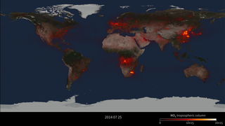
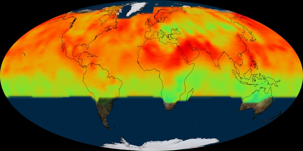
Nitrogen Dioxide from Aura/OMI, 2013-2014
Go to this sectionThis yearlong timeseries of NO₂ from OMI run from July 2013 to July 2014.
- Section
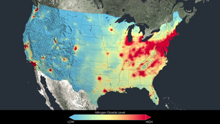
NASA Images Highlight U.S. Air Quality Improvement – Release Materials
Go to this sectionThis visualization corresponds to a hyperwall show of the material above.
- Section
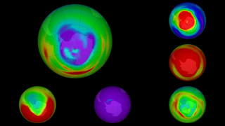
Montage of early data from Aura's Microwave Limb Sounder
Go to this sectionMontage of six measurements made by MLS
- Section
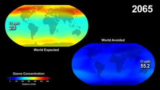
What Would have Happened to the Ozone Layer if Chlorofluorocarbons (CFCs) had not been Regulated? (UPDATED)
Go to this sectionWorld Avoided Ozone Full Animation
- Section

Monthly Carbon Monoxide (Terra/MOPITT)
Go to this sectionMonthly Terra/MOPITT carbon monoxide maps, March 2000 to the present.
- Section
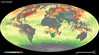
Monthly Aerosol Particle Radius (Aqua/MODIS)
Go to this sectionMonthly Aqua/MODIS aerosol particle radius, July 2002 to the present.
- Section
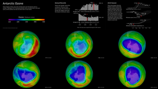
OzoneWatch: status of the ozone layer over the Antarctic
Go to this sectionOzone hole size plots and October 1st images from 1979-2014
- ID: 4402 Visualization
A Year of Global Carbon Dioxide Measurements
Go to this pageMollweide projected animation of CO2 data from the OCO-2 mission. Data spans from September 2014 to August 2015. As the data cycles through the year, you can see an increase CO2 concentrations across the northern hemisphere going from winter to spring. Then in the summer, as vegetation reaches it's peak, there is a noticeable decline in CO2 concentration throughout the entire northern hemisphere. || global_oco2_flat4k.0700.mollweide_print.jpg (1024x512) [90.2 KB] || global_oco2_flat4k.0700.mollweide_searchweb.png (180x320) [60.4 KB] || global_oco2_flat4k.0700.mollweide_thm.png (80x40) [5.9 KB] || global_oco2_mollweide4k_1080p30.mp4 (1920x1080) [10.0 MB] || global_oco2_mollweide4k_1080p30.webm (1920x1080) [2.8 MB] || oco2_mollweide_w_dates_1080p30.mp4 (1920x1080) [10.1 MB] || global_oco2_mollweide4k_2160p30.mp4 (4320x2160) [34.1 MB] || mollweide (4320x2160) [0 Item(s)] || mollweide_with_dates (3840x2160) [0 Item(s)] || oco2_mollweide_w_dates_2160p30.mp4 (3840x2160) [30.5 MB] || oco2_mollweide_w_dates_4402.key [14.1 MB] || oco2_mollweide_w_dates_4402.pptx [11.5 MB] || global_oco2_mollweide4k_1080p30.mp4.hwshow [197 bytes] || oco2_mollweide_w_dates_1080p30.mp4.hwshow [232 bytes] ||
Weather
The Earth’s weather system includes the dynamics of the atmosphere and its interaction with the oceans and land. Weather ranges from local or microphysical processes that occur in minutes through global-scale phenomena that we can predict with a degree of success at an estimated maximum of two weeks prior.
- Section
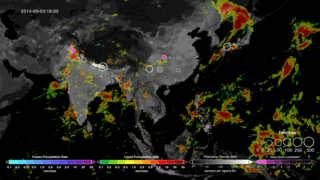
Global Rainfall-Triggered Landslides and Global Precipitation from IMERG
Go to this sectionThis visualization shows rainfall-triggered landslides and precipitation from August and September of 2014 in Asia and the Himalayan Arc.
- Section
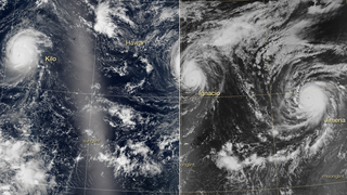
Trio of Hurricanes Over the Pacific Ocean
Go to this sectionTrio of Hurricanes Over the Pacific Ocean
Climate Variability & Change
NASA’s Climate Variability and Change Focus Area studies global climate and sea level to understand their change on seasonal to decadal timescales. Home to NASA’s research programs in Physical Oceanography, Cryospheric Sciences, and Modeling and Data Assimilation, this focus area fosters interdisciplinary science to understand the role of oceans and ice in the Earth system, and supports advanced modeling capabilities to improve our understanding of the physical processes that control the earth system and enable prediction.
- Section

El Niño Watch 2015
Go to this sectionAnimation of Sea Surface Height Anomaly for 2015 compared to 1997
- ID: 30515 Hyperwall Visual
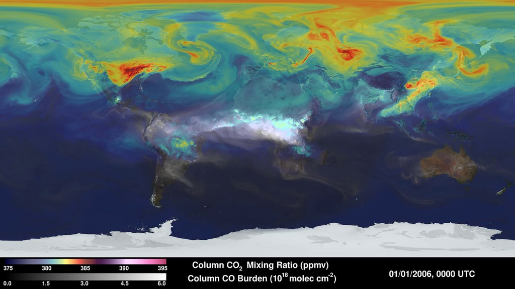
Simulated Atmospheric Carbon Concentrations
Go to this pageCarbon exists in many forms—e.g., carbon dioxide (CO2), carbon monoxide (CO)—and continually cycles through Earth’s atmosphere, ocean, and terrestrial ecosystems. This visualization, created using data from the 7-km GEOS-5 Nature Run model, shows average column concentrations of atmospheric CO2 (colored shades) and CO (white shades underneath) from January 1, 2006 to December 31, 2006.CO2 variations are largely controlled by fossil fuel emissions and seasonal fluxes of carbon between the atmosphere and land biosphere. For example, dark red and pink shades represent regions where CO2 concentrations are enhanced by carbon sources, mainly from human activities. During Northern Hemisphere spring and summer months, plants absorb a substantial amount of CO2 through photosynthesis, thus removing CO2 from the atmosphere. Atmospheric CO, a pollutant harmful to human health, is produced mainly from fossil fuel combustion and biomass burning. Here, high concentrations of CO (white) are mainly from fire activity in Africa, South America, and Australia. Scientists use model output data such as these to help answer important questions about Earth’s climate and to help design future satellite missions.These model simulations use fossil fuel emissions estimates provided by the Emissions Database for Global Atmospheric Research (EDGAR). NASA’s Quick Fire Emissions Dataset (QFED) estimates fire emissions using MODIS fire radiative power observations. Additional, observationally constrained estimates of CO2 flux between the atmosphere and land and ocean carbon reservoirs were produced as part of NASA’s Carbon Monitoring System Flux Pilot Project (http://carbon.nasa.gov/cgi-bin/cms/inv_pgp.pl?pgid=581). Land biosphere fluxes come from the Carnegie-Ames-Stanford Approach Global Fire Emissions Database (CASA-GFED) model which incorporates MODIS vegetation classification and AVHRR Normalized Difference Vegetation Index (NDVI) data. Ocean fluxes are produced by the NASA Ocean Biogeochemical Model (NOBM) which incorporates MODIS chlorophyll observations. ||
- ID: 30604 Hyperwall Visual
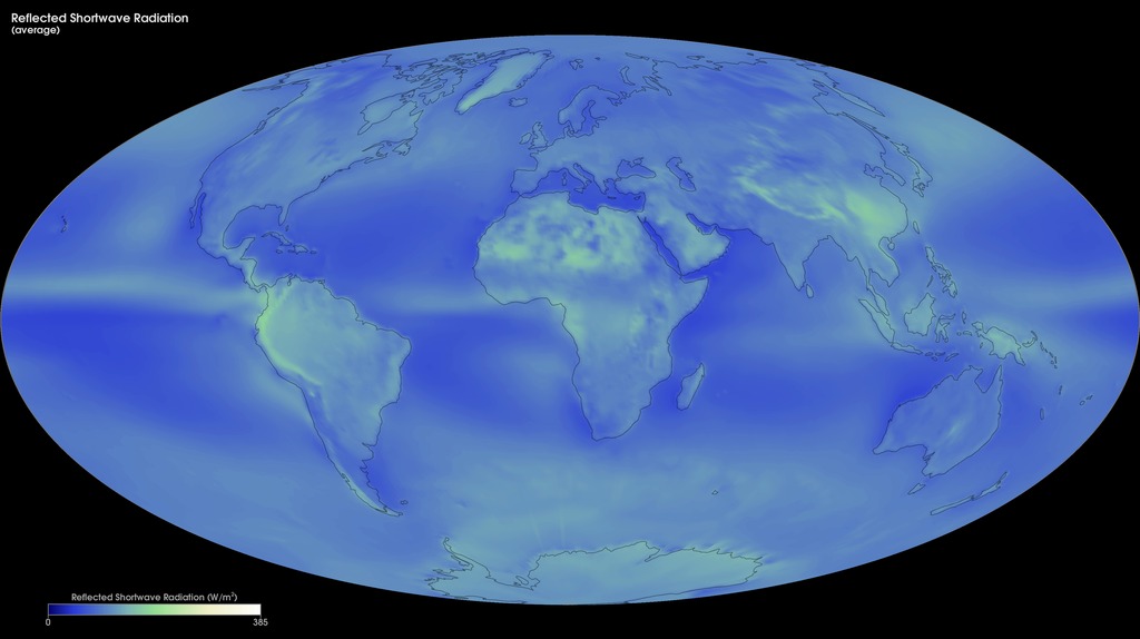
CERES Radiation Fluxes
Go to this pageThese maps show monthly reflected-shortwave radiation from March 2000 to the present from the Energy Balanced and Filled (EBAF) data product. These data are produced by averaging observations collected by the Clouds and the Earth's Radiant Energy System (CERES) sensors on NASA's Aqua and Terra satellites, filling in gaps and constraining the fluxes to remove the inconsistency between average global net TOA flux and heat storage in the Earth-atmosphere system. ||
- ID: 30603 Hyperwall Visual
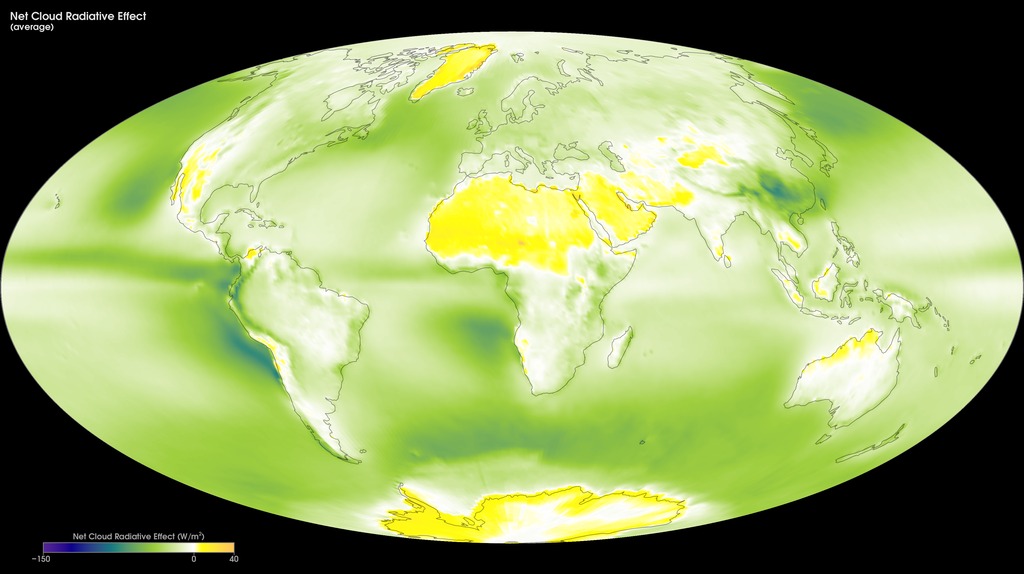
CERES Cloud Radiative Effect
Go to this pageCERES Net Cloud Radiative Effect || ceres_net_cre_average_2000-2015_print.jpg (1024x574) [102.2 KB] || ceres_net_cre_average_2000-2015.png (4104x2304) [2.1 MB] || ceres_net_cre_average_2000-2015_searchweb.png (320x180) [69.4 KB] || ceres_net_cre_average_2000-2015_thm.png (80x40) [6.5 KB] || ceres_net_cre_average_2000-2015_30603.pptx [3.0 MB] || ceres_net_cre_average_2000-2015_30603.key [5.6 MB] ||
Water & Energy Cycle
The Water and Energy Cycle Focus Area seeks to enhance our understanding of the transfer and storage of water and energy in the Earth system. For the water cycle, the emphasis is on atmospheric and terrestrial stores, including seasonal snow cover. Permanent snow and ice, as well as ocean dynamics, are studied within the Climate Variability and Change Focus Area. The Water and Energy Cycle Focus Area aims to resolve all fluxes of water and the corresponding energy fluxes involved with the water changing phase. High priority is placed on understanding, observing, and modeling clouds and their interaction with energy fluxes
- Section
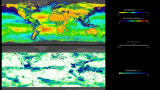
Soil Moisture and Rainfall
Go to this sectionSoil Moisture and Ocean Salinity are compared to Rainfall
- Section
- Section
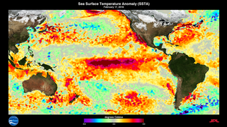
ENSO Sea Surface Temperature Anomalies: 2015-2016
Go to this sectionAnimation of Sea Surface Temperature shows the evolution of the 2015-2016 ENSO event.
- ID: 4353 Visualization

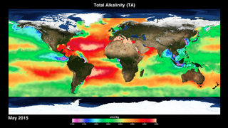
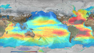
Aquarius Sea Surface Salinity 2011-2015
Go to this pageRectangular flat map projection shows Sea Surface Salinity measurements taken by Aquarius in its whole life span (September 2011 - May 2015). || aquarius_sss_timeCbar_flatmap_1080p30_print.jpg (1024x576) [137.4 KB] || aquarius_sss_timeCbar_flatmap_1080p30_searchweb.png (320x180) [80.4 KB] || aquarius_sss_timeCbar_flatmap_1080p30_web.png (320x180) [80.4 KB] || aquarius_sss_timeCbar_flatmap_1080p30_thm.png (80x40) [7.2 KB] || aquarius_sss_timeCbar_flatmap_1080p30.mp4 (1920x1080) [83.1 MB] || aquarius_sss_timeCbar_flatmap_1080p30.webm (1920x1080) [12.0 MB] || flatmap_4k (3840x2160) [0 Item(s)] || flatmap_no_timeCbar_4k (3840x2160) [0 Item(s)] || aquarius_sss_timeCbar_flatmap_4353.key [88.0 MB] || aquarius_sss_timeCbar_flatmap_4353.pptx [85.4 MB] || aquarius_sss_timeCbar_flatmap_4k_2160p30.mp4 (3840x2160) [259.0 MB] || aquarius-sea-surface-salinity-2011-2015.hwshow [203 bytes] ||
- Section
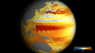
22-year Sea Level Rise - TOPEX/JASON
Go to this sectionSpinning globe showing TOPEX/JASON 22-year sea level data. Earth spins once before camera zooms into West Atlantic, East Pacific, and West Pacific regions. With colorbar
- Section
Cryosphere
- Section

Greenland's Glaciers as seen by RadarSat
Go to this sectionAn animation up the Greenland's Sermilik Fjord to the calving front of the Helheim Glacier, showing the glacier front's change between 2000 to 2013
- Section

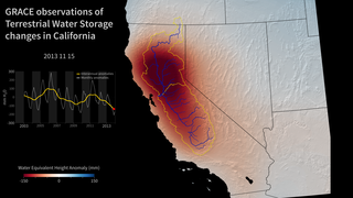
NASA GSFC MASCON Solution over Greenland from Jan 2004 - Jun 2014
Go to this sectionVisualization of the mass change over Greenland from January 2004 through June 2014. The surface of Greenland shows the change in equivalent water height while the graph overlay shows the total accumulated change in gigatons.
- Section

Antarctic Mass Change from GRACE derived Gravity Observations: Jan 2004 - Jun 2014
Go to this sectionAn animation of mass change over the Antarctic Ice Sheet from GRACE derived gravity observations.
- Section
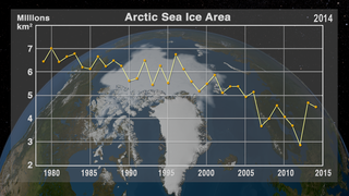
Annual Arctic Sea Ice Minimum 1979-2014 with Area Graph
Go to this sectionThis animation shows the annual Arctic sea ice minimum with a graph overlay that depicts the area of the sea ice in millions of square kilometers.
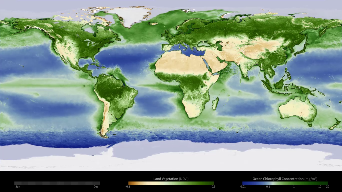
Carbon Cycle & Ecosystems
The Earth's ecosystems and biogeochemical cycles (such as carbon, nitrogen, and phosphorus) both drive and respond to environmental changes ranging from local to global scales. These environmental changes are occurring on an unprecedented scale, in both time and geographical extent. Major uncertainties in Earth science originate from the dynamics and interactions within and between ecosystems and biogeochemical cycles across land, ocean, atmospheric, and human systems.
- ID: 30595 Hyperwall Visual
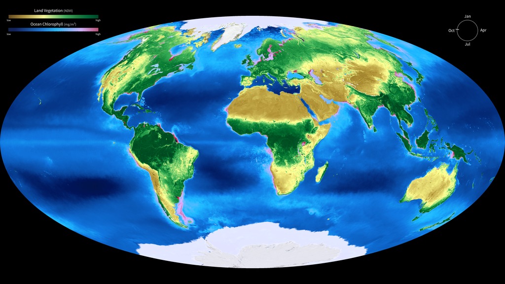
Global Biosphere, Yearly Cycle
Go to this pageA different color scheme to differentiate ocean and land. || biosphere_cryo_280_print.jpg (1024x576) [145.4 KB] || biosphere_cryo_280_searchweb.png (180x320) [77.2 KB] || biosphere_cryo_280_thm.png (80x40) [7.2 KB] || biosphere_cryo_1080p.mp4 (1920x1080) [10.5 MB] || biosphere_cryo_720p.mp4 (1280x720) [5.0 MB] || biosphere_cryo_720p.webm (1280x720) [1.4 MB] || biosphere_cryo_2160p.mp4 (3840x2160) [37.2 MB] || biosphere_cryo_280.tif (5760x3240) [14.7 MB] || biosphere_cryo_3240p.mp4 (5760x3240) [43.6 MB] || biosphere_cryo_30595.key [14.6 MB] || biosphere_cryo_30595.pptx [12.0 MB] ||
- ID: 30601 Hyperwall Visual

SMAP's First High-Resolution Global Soil Moisture Map
Go to this pageA global map of soil moisture || smap_global_moisture_20150504-20150511_PIA19337_print.jpg (1024x576) [113.1 KB] || smap_global_moisture_20150504-20150511_PIA19337.png (5760x3240) [5.3 MB] || smap_global_moisture_20150504-20150511_PIA19337_searchweb.png (320x180) [43.4 KB] || smap_global_moisture_20150504-20150511_PIA19337_thm.png (80x40) [4.7 KB] || smap_global_moisture_30601.pptx [5.8 MB] || smap_global_moisture_30601.key [8.5 MB] || smap_global_moisture_20150504-20150511_PIA19337.hwshow [262 bytes] ||
- Section
- ID: 30709 Hyperwall Visual
Yearly Cycle of Earth's Biosphere
Go to this pageanimation with traditional colors for chl || yearly_biosphere_color2_1080p.00001_print.jpg (1024x576) [164.5 KB] || yearly_biosphere_color2_1080p.00001_searchweb.png (180x320) [86.0 KB] || yearly_biosphere_color2_1080p.00001_thm.png (80x40) [6.9 KB] || yearly_biosphere_color2_1080p.mp4 (1920x1080) [17.2 MB] || yearly_biosphere_color2_1080p.webm (1920x1080) [1.3 MB] || yearly_biosphere_color2_1080p.hwshow [94 bytes] ||
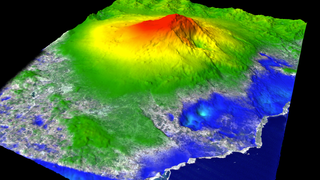
Earth Surface & Interior
The overarching goal of Earth's surface and Interior focus is to use NASA’s unique capabilities and observational resources to better understand core, mantle, and lithospheric structure and dynamics, and interactions between these processes and Earth’s fluid envelopes.
- Section
- Section
- Section
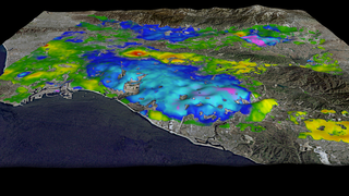
Southern California Groundwater
Go to this sectionRadar reveals changes in Southern California groundwater.
- Section
Models
GEOS, ECCO, climate models, etc
- Section
- Section
Modeled Phytoplankton Communities in the Global Ocean
Go to this sectionA rotating globe shows the distribution of phytoplankton the the world's oceans
- Section
AXIOM-1 Sea Surface Salinity, Sea Ice Thickness and Atmospheric Precipitable Water
Go to this sectionThis animation shows sea surface sailinity, sea ice thickness, and atmospheric precipitable water.