The Curious World of Scientific Visualization
Overview
Explore data brought to life by NASA’s artists and scientists
Data Brought to Life
Data is only as powerful as our ability to make sense of it. The right tools can help us find meaning in a trove of information and experience the wonder in it. When artists and scientists work in concert, they unearth stories within datasets and push the boundaries of knowledge. This collaboration is both a creative process and a mathematical one. Scientific visualization is not a mere translation of numbers into pictures: shapes and colors breathe life into real scientific data, allowing us to see patterns and complexities that were once invisible or unknown. The visualization itself becomes a vehicle for scientific inquiry, capturing the curiosity of both artist and scientist. When shared with the world, these data-driven artworks inspire as much as they educate and entertain. Scientific visualization reminds us of the beauty in understanding, and it is a means of discovery all its own.
Scientific Visualization at NASA
At NASA’s Goddard Space Flight Center, scientists work alongside a team of artists to extend their research into the visual space. The Scientific Visualization Studio creates animations and videos that showcase the latest discoveries in Earth and space sciences. These visualizations are both insightful tools for the NASA research community and accessible science stories designed to be enjoyed by people of all walks of life. As one of NASA’s leading outreach efforts, the Scientific Visualization Studio empowers scientists to share their work with as wide an audience as possible, in the most creative and engaging way possible.
Introductory Gallery
Visualizations which exempilfy the vast reach of our work and which set the stage for the stories we want to tell in the other galleries.
- ID: 11003 Produced Video
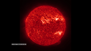
Excerpt from "Dynamic Earth"
Go to this pageA giant explosion of magnetic energy from the sun, called a coronal mass ejection, slams into and is deflected completely by the Earth's powerful magnetic field. The sun also continually sends out streams of light and radiation energy. Earth's atmosphere acts like a radiation shield, blocking quite a bit of this energy.Much of the radiation energy that makes it through is reflected back into space by clouds, ice and snow and the energy that remains helps to drive the Earth system, powering a remarkable planetary engine — the climate. It becomes the energy that feeds swirling wind and ocean currents as cold air and surface waters move toward the equator and warm air and water moves toward the poles — all in an attempt to equalize temperatures around the world.A jury appointed by the National Science Foundation (NSF) and Science magazine has selected "Excerpt from Dynamic Earth" as the winner of the 2013 NSF International Science and Engineering Visualization Challenge for the Video category. This animation will be highlighted in the February 2014 special section of Science and will be hosted on ScienceMag.org and NSF.govThis animation was selected for the Computer Animation Festival's Electronic Theater at the Association for Computer Machinery's Special Interest Group on Computer Graphics and Interactive Techniques (SIGGRAPH), a prestigious computer graphics and technical research forum. This is an excerpt from the fulldome, high-resolution show 'Dynamic Earth: Exploring Earth's Climate Engine.' The Dynamic Earth dome show was selected as a finalist in the Jackson Hole Wildlife Film Festival Science Media Awards under the category "Best Immersive Cinema - Fulldome". ||
- ID: 4583 Visualization
NASA's Near-Earth Science Mission Fleet: March 2017
Go to this pageNASA Near-Earth Science Fleet (August 2017) || near_earth_sciences02.6100_print.jpg (1024x576) [69.3 KB] || near_earth_sciences02.6100_searchweb.png (320x180) [44.2 KB] || near_earth_sciences02.6100_thm.png (80x40) [4.0 KB] || near_earth_sciences02_1080p60.mp4 (1920x1080) [51.2 MB] || 1920x1080_16x9_60p (1920x1080) [0 Item(s)] || near_earth_sciences02_1080p60.webm (1920x1080) [12.6 MB] || near_earth_sciences02_360p30.mp4 (640x360) [6.6 MB] || 9600x3240_16x9_30p (9600x3240) [0 Item(s)] ||
- Section

Hyperwall
Go to this sectionThis is a placeholder for a potential video of a presentation in the hyperwall room, maybe even a 360 video of one of us presenting.
- ID: 11719 Produced Video
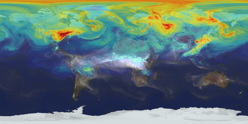
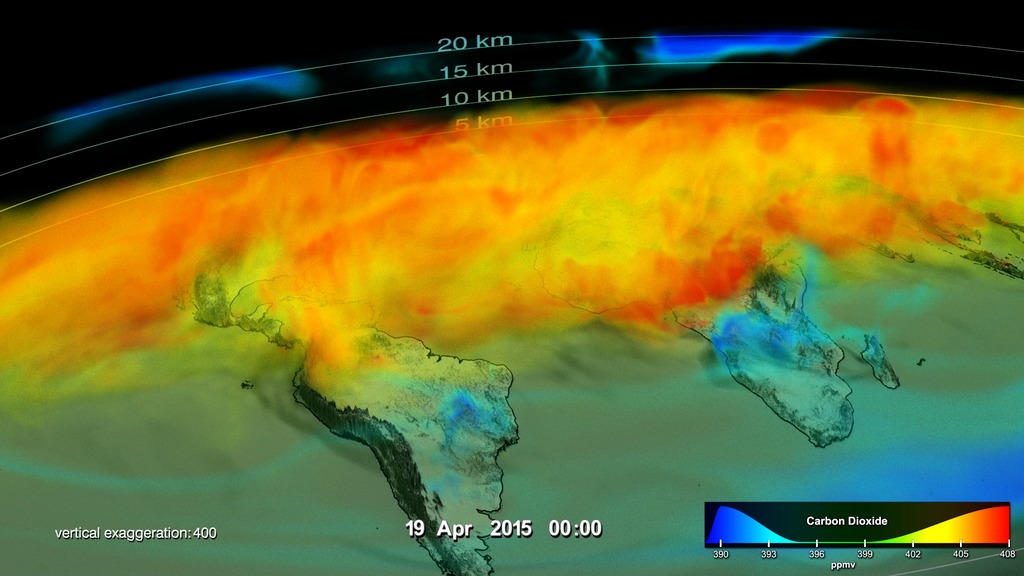
A Year In The Life Of Earth’s CO2
Go to this pageAn ultra-high-resolution NASA computer model has given scientists a stunning new look at how carbon dioxide in the atmosphere travels around the globe.Plumes of carbon dioxide in the simulation swirl and shift as winds disperse the greenhouse gas away from its sources. The simulation also illustrates differences in carbon dioxide levels in the northern and southern hemispheres and distinct swings in global carbon dioxide concentrations as the growth cycle of plants and trees changes with the seasons.The carbon dioxide visualization was produced by a computer model called GEOS-5, created by scientists at NASA Goddard Space Flight Center’s Global Modeling and Assimilation Office.The visualization is a product of a simulation called a “Nature Run.” The Nature Run ingests real data on atmospheric conditions and the emission of greenhouse gases and both natural and man-made particulates. The model is then left to run on its own and simulate the natural behavior of the Earth’s atmosphere. This Nature Run simulates January 2006 through December 2006.While Goddard scientists worked with a “beta” version of the Nature Run internally for several years, they released this updated, improved version to the scientific community for the first time in the fall of 2014. ||
- Section
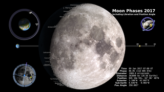
Moon Phase and Libration, 2017
Go to this sectionA lot of information in a beautiful visualization.
Beauty and Understanding
It’s often the beauty of a visualization that commands our attention. At first, a visualization may seem more like a wildly imaginative piece of art than a representation of concrete scientific observations. The rhythm of the colors, shapes and motions is so wondrous we don’t expect it to be real, but its realness is actually the most beautiful part of it all. A beautiful visualization invites us to venture to a place of deeper understanding, and a profound appreciation comes with the realization that we can learn from its elegance.
Look for: Meaning in swaths of color, processes as patterns
Original Caption: Visualizations are beautiful because the story they tell is real. Understanding enhances appreciation in these cases.
- ID: 3827 Visualization
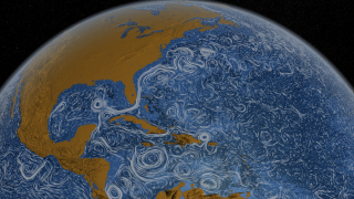
Perpetual Ocean
Go to this pageThis visualization shows ocean surface currents around the world during the period from June 2005 through December 2007. The visualization does not include a narration or annotations; the goal was to use ocean flow data to create a simple, visceral experience.This visualization was produced using model output from the joint MIT/JPL project: Estimating the Circulation and Climate of the Ocean, Phase II or ECCO2. ECCO2 uses the MIT general circulation model (MITgcm) to synthesize satellite and in-situ data of the global ocean and sea-ice at resolutions that begin to resolve ocean eddies and other narrow current systems, which transport heat and carbon in the oceans. ECCO2 provides ocean flows at all depths, but only surface flows are used in this visualization. The dark patterns under the ocean represent the undersea bathymetry. Topographic land exaggeration is 20x and bathymetric exaggeration is 40x. This visualization was shown at the SIGGRAPH Asia 2012 Computer Animation Festival.Don't miss these related visualizations:Excerpt form Dynamic EarthGulf Stream Sea Surface Currents and TemperaturesOcean Current Flows around the Mediterranean Sea for UNESCOGlobal Sea Surface Currents and TemperatureFlat Map Ocean Current Flows with Sea Surface Temperatures (SST) ||
- ID: 3354 Visualization

27 Storms: Arlene to Zeta
Go to this pageMany records were broken during the 2005 Atlantic hurricane season including the most hurricanes ever, the most category 5 hurricanes, and the most intense hurricane ever recorded in the Atlantic as measured by atmospheric pressure. This visualization shows all 27 named storms that formed in the 2005 Atlantic hurricane season and examines some of the conditions that made hurricane formation so favorable.The animation begins by showing the regions of warm water that are favorable for storm development advancing northward through the peak of hurricane season and then receding as the waters cool. The thermal energy in these warm waters powers the hurricanes. Strong shearing winds in the troposphere can disrupt developing young storms, but measurements indicate that there was very little shearing wind activity in 2005 to impede storm formation.Sea surface temperatures, clouds, storm tracks, and hurricane category labels are shown as the hurricane season progresses.This visualization shows some of the actual data that NASA and NOAA satellites measured in 2005 — data used to predict the paths and intensities of hurricanes. Satellite data play a vital role in helping us understand the land, ocean, and atmosphere systems that have such dramatic effects on our lives.NOTE: This animation shows the named storms from the 2005 hurricane season. During a re-analysis of 2005, NOAA's Tropical Prediction Center/National Hurricane Center determined that a short-lived subtropcial storm developed near the Azores Islands in late September, increasing the 2005 tropical storm count from 27 to 28. This storm was not named and is not shown in this animation.'27 Storms: Arlene to Zeta' played in the SIGGRAPH 2007 Computer Animation Festival in August 2007. It was also a finalist in the 2006 NSF Science and Engineering Visualization Challenge. ||
- ID: 4455 Visualization
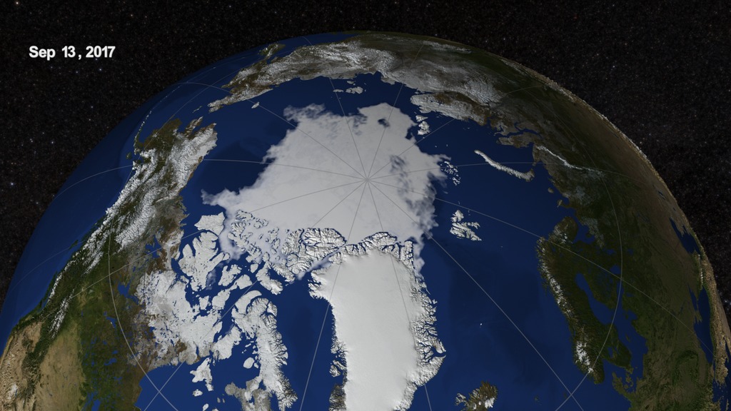
Arctic Sea Ice from March to September 2017
Go to this pageIn this visualization, the daily Arctic sea ice and seasonal land cover change progress through time, from this year’s wintertime maximum extent on March 7, 2017, through September 13, 2017 when the sea ice reached its annual minimum extent for the year. Over the water, Arctic sea ice changes from day to day showing a running 3-day minimum sea ice concentration in the region where the concentration is greater than 15%. The blueish white color of the sea ice is derived from a 3-day running minimum of the AMSR2 89 GHz brightness temperature. Over the terrain, monthly data from the seasonal Blue Marble Next Generation fades slowly from month to month. || SeaIceMin2017_1920x1080_print.jpg (1024x576) [161.8 KB] || SeaIceMin2017_1920x1080_searchweb.png (320x180) [98.0 KB] || SeaIceMin2017_1920x1080_thm.png (80x40) [6.7 KB] || 1920x1080_16x9_60p (1920x1080) [0 Item(s)] || 1920x1080_16x9_30p (1920x1080) [0 Item(s)] || SeaIceMin2017_30fps_1080p30.mp4 (1920x1080) [22.0 MB] || SeaIceMin2017_1920x1080.tif (1920x1080) [3.3 MB] || SeaIceMin2017_30fps_1080p30.webm (1920x1080) [1.5 MB] || SeaIceMin2017_30fps_1080p30.mp4.hwshow [193 bytes] ||
- ID: 30637 Hyperwall Visual

GEOS-5 Aerosols Simulation for SC 2014
Go to this pageGEOS-5 aerosols shown at SC 2014. || aerosols-sc2014-preview.jpg (1024x512) [140.7 KB] || aerosols_globe_c1440_NR_BETA9-SNAP_20070228_2200z_searchweb.png (180x320) [97.6 KB] || aerosols_globe_c1440_NR_BETA9-SNAP_20070228_2200z_thm.png (80x40) [7.4 KB] || aerosols (1920x1080) [0 Item(s)] || aerosols-sc14.webm (1920x1080) [10.2 MB] || aerosols-sc14.mp4 (1920x1080) [155.5 MB] || 30637_aerosols_sim_1920x1080.mp4 (1920x1080) [204.3 MB] || aerosols (5760x2881) [0 Item(s)] || 30637_aerosols_sim_4K.mp4 (4096x2048) [206.8 MB] || 30637_aerosols_sim_UHD_large.mp4 (3840x2160) [206.3 MB] || 30637_aerosols_sim_1280x720_prores.mov (1280x720) [1.5 GB] || 30637_aerosols_sim_UHD_youtube_hq.mov (3840x2160) [4.0 GB] || 30637_aerosols_sim_UHD.mov (3840x2160) [11.2 GB] || 30637_aerosols_sim_MASTER.mov (5760x2881) [23.5 GB] ||
- ID: 4596 Visualization
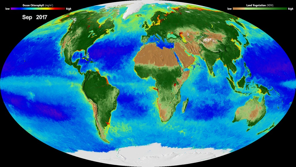
20 Years of Global Biosphere (updated)
Go to this pageThis Mollweide projected data visualization shows 20 years of Earth's biosphere starting in September 1997 going through September 2017. Data for this visualization was collected from multiple satellites over the past twenty years. || biosphere7_mollweide.4507_print.jpg (576x1024) [192.2 KB] || biosphere7_mollweide.4507_searchweb.png (180x320) [91.0 KB] || biosphere7_mollweide.4507_thm.png (80x40) [7.4 KB] || mollweide_annotated (1920x1080) [0 Item(s)] || biosphere7_mollweide_1080p30.webm (1920x1080) [17.8 MB] || biosphere7_mollweide_1080p30.mp4 (1920x1080) [264.8 MB] || biosphere7_mollweide_1080p30.mp4.hwshow ||
Making the Invisible Visible
Visualization is the process of making something visible that was not visible before. For a scientist, this might mean looking at something in a frequency that the human eye cannot see or looking through a cloud to see the rainfall inside. For a visualizer, it could mean viewing a property that the mind can understand but the eye cannot see, such as the currents in an ocean or the ozone in the atmosphere.
- ID: 4128 Visualization

Solar Dynamics Observatory - Argo view - Slices of SDO
Go to this pageArgos (or Argus Panoptes) was the 100-eyed giant in Greek mythology (wikipedia).While the Solar Dynamics Observatory (SDO) has significantly less than 100 eyes, (see "SDO Jewelbox: The Many Eyes of SDO"), seeing connections in the solar atmosphere through the many filters of SDO presents a number of interesting challenges. This visualization experiment illustrates a mechanism for highlighting these connections. This visualization is a variation of the original Solar Dynamics Observatory - Argo view. In this case, the different wavelength filters are presented in three sets around the Sun at full 4Kx4K resolution. This enables monitoring of changes in time over all wavelengths at any location around the limb of the Sun. The wavelengths presented are: 617.3nm optical light from SDO/HMI. From SDO/AIA we have 170nm (pink), then 160nm (green), 33.5nm (blue), 30.4nm (orange), 21.1nm (violet), 19.3nm (bronze), 17.1nm (gold), 13.1nm (aqua) and 9.4nm (green).We've locked the camera to rotate the view of the Sun so each wedge-shaped wavelength filter passes over a region of the Sun. As the features pass from one wavelength to the next, we can see dramatic differences in solar structures that appear in different wavelengths.Filaments extending off the limb of the Sun which are bright in 30.4 nanometers, appear dark in many other wavelengths.Sunspots which appear dark in optical wavelengths, are festooned with glowing ribbons in ultraviolet wavelengths.small flares, invisible in optical wavelengths, are bright ribbons in ultraviolet wavelengths.if we compare the visible light limb of the Sun with the 170 nanometer filter on the left, with the visible light limb and the 9.4 nanometer filter on the right, we see that the 'edge' is at different heights. This effect is due to the different amounts of absorption, and emission, of the solar atmosphere in ultraviolet light.in far ultraviolet light, the photosphere is dark since the black-body spectrum at a temperature of 5700 Kelvin emits very little light in this wavelength. ||
- ID: 11491 Produced Video
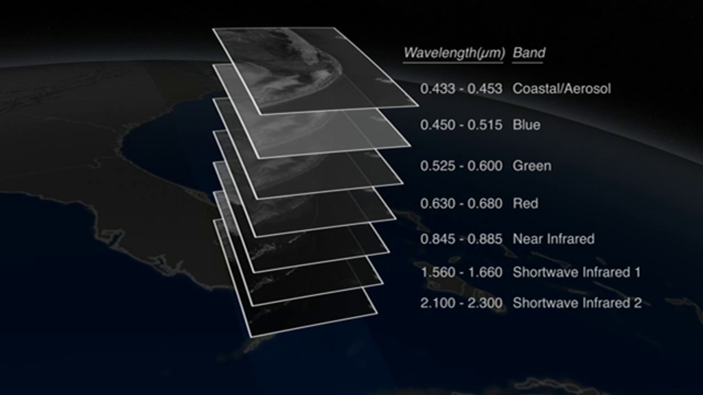
Landsat 8 Onion Skin
Go to this pageLandsat satellites circle the globe every 99 minutes, collecting data about the land surfaces passing underneath. After 16 days, the Landsat satellite has passed over every spot on the globe, and recorded data in 11 different wavelength regions. The individual wavelength bands can be combined into color images, with different combinations of the 11 bands revealing different information about the condition of the land cover.The data for this video was collected by Landsat 5 on November 10, 2011. ||
- ID: 4458 Visualization
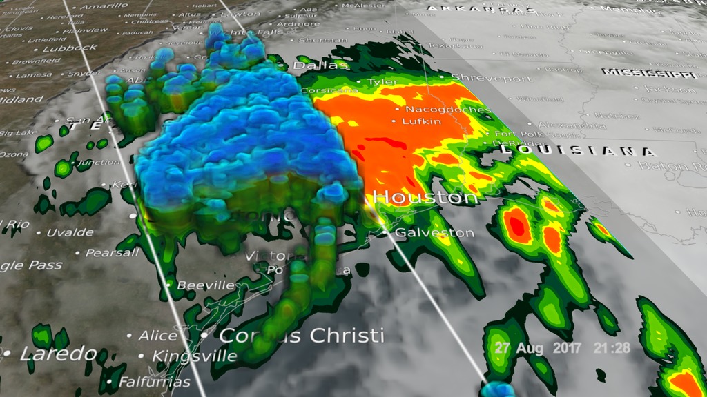
Harvey Floods Texas and Threatens Louisiana (Final Tropical Storm Update)
Go to this pageGPM caught Tropical Storm Harvey twice on August 30th, 2017. This time the storm made landfall in Louisiana and moved up east of the Texas/Louisiana border pounding already drenched eastern Texas and western Louisiana with more rain. || harvey_v2.3400_print.jpg (1024x576) [163.6 KB] || harvey_v3.mp4 (1920x1080) [91.1 MB] || harvey_through_aug_30 (1920x1080) [128.0 KB] || harvey_v3.webm (1920x1080) [11.4 MB] || GSFC_20170830_GPM_m4458_Harvey.en_US.vtt [64 bytes] || harvey.mp4.hwshow [187 bytes] ||
- ID: 3912 Visualization
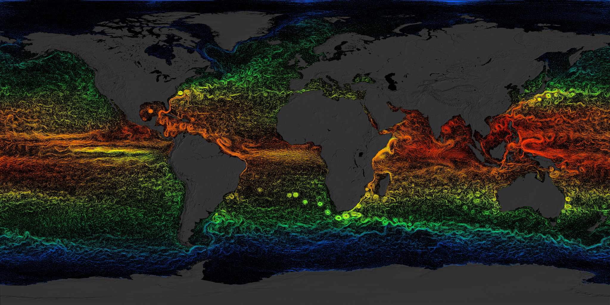
Global Sea Surface Currents and Temperature
Go to this pageThis visualization shows sea surface current flows. The flows are colored by corresponding sea surface temperature data. This visualization is rendered for display on very high resolution devices like hyperwalls or for print media.This visualization was produced using model output from the joint MIT/JPL project entitled Estimating the Circulation and Climate of the Ocean, Phase II (ECCO2). ECCO2 uses the MIT general circulation model (MITgcm) to synthesize satellite and in-situ data of the global ocean and sea-ice at resolutions that begin to resolve ocean eddies and other narrow current systems, which transport heat and carbon in the oceans. The ECCO2 model simulates ocean flows at all depths, but only surface flows are used in this visualization. ||
- ID: 4160 Visualization
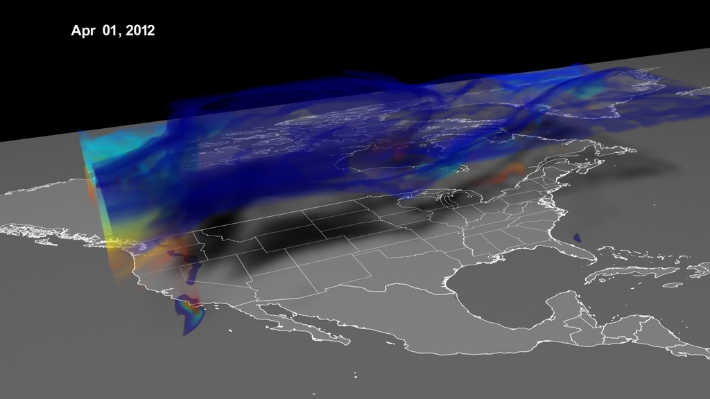
Stratospheric Ozone Intrusion
Go to this pageEvents called stratospheric ozone intrusions occur most often in spring and early summer, and can raise ground-level ozone concentrations in some areas to potentially unhealthy levels.This visualization shows one such event that occurred on April 6, 2012. On that day, a fast-moving area of low pressure moved northeast across states in the Western U.S., clipping western and northern Colorado. Ozone-rich stratospheric air descended, folding into tropospheric air near the ground. Winds took hold of the air mass and pushed it in all directions, bringing stratospheric ozone to the ground in Colorado and along the Northern Front Range.Atmospheric scientists at NASA's Goddard Space Flight Center in Greenbelt, Md., set out to see if the Goddard Earth Observing System Model, Version 5 (GEOS-5) Chemistry-Climate Model could replicate stratospheric ozone intrusions at 25-kilometer (16-mile) resolution. High-resolution models are possible due to computing power now capable of simulating the chemistry and movement of gasses and pollutants around the atmosphere and calculating their interactions.They show that indeed, the model could replicate small-scale features, including finger-like filaments, within the apron of ozone-rich stratospheric air that descended over Colorado on April 6, 2012. ||
Fitting Data Together
Visualizations of complex systems often use either multiple datasets or long term data records to explain hidden phenomena.
- ID: 4283 Visualization
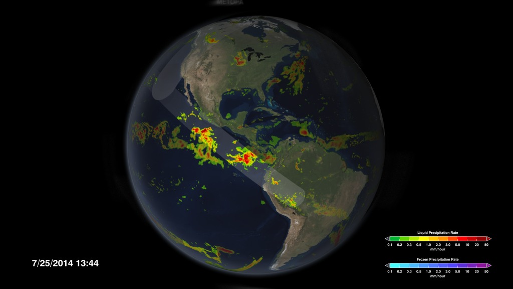
Painting the World with Water
Go to this pageAn animation depicting the build-up of precipitation data on the globe from the Global Precipitation Measurement constellation of satellites, resulting in the IMERG global precipitation data set. || GPM_Fleet_IMERG_globe.00556_print.jpg (1024x576) [66.4 KB] || GPM_Fleet_IMERG_globe.00556_searchweb.png (180x320) [41.1 KB] || GPM_Fleet_IMERG_globe.00556_web.png (320x180) [41.1 KB] || GPM_Fleet_IMERG_globe.00556_thm.png (80x40) [3.7 KB] || GPM_Fleet_IMERG_globe.webm (1920x1080) [5.8 MB] || GPM_Fleet_IMERG_globe.mp4 (1920x1080) [55.2 MB] || globecomposite (1920x1080) [128.0 KB] || GPM_Fleet_IMERG_globe_4283.pptx [55.9 MB] || GPM_Fleet_IMERG_globe_4283.key [58.4 MB] || GPM_Fleet_IMERG_globe.mp4.hwshow [214 bytes] ||
- ID: 4573 Visualization
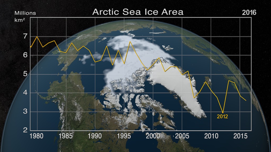
Annual Arctic Sea Ice Minimum 1979-2016 with Area Graph
Go to this pageA visualization of the annual minimum Arctic sea ice from 1979 to 2016 with a graph overlay. (fast playback)This video is also available on our YouTube channel. || seaIceWgraph_2016_p30.0568_print.jpg (1024x576) [168.2 KB] || seaIceWgraph_2016_fast_1080p30.mp4 (1920x1080) [2.6 MB] || seaIceWgraph_2016_fast_1080p30.webmhd.webm (1080x606) [1.8 MB] || seaIceWgraph_2016_fast_2160p30.mp4 (3840x2160) [7.1 MB] || seaIce_withGraph (3840x2160) [0 Item(s)] || seaIceWgraph_2016_fast_1080p30.mp4.hwshow [196 bytes] ||
- ID: 4575 Visualization

NASA Studies Hurricane Matthew
Go to this pageThis data visualization follows Hurricane Matthew throughout its destructive run in the Caribbean and Southeast U.S. coast. By utilizing different data sets from NOAA's GOES satellite, NASA/JAXA's GPM, MERRA-2 model runs, IMERG, Goddard's soil moisture product, and sea surface temperatures, scientists are able to put together a clearer picture of how this hurricane quickly intensified and eventually weakened. || matthew_narrated_v106.5800_print.jpg (1024x576) [189.6 KB] || matthew_narrated_v106.5800_searchweb.png (320x180) [114.8 KB] || matthew_narrated_v106.5800_thm.png (80x40) [7.8 KB] || matthew (1920x1080) [0 Item(s)] || matthew_narrated_v106.webm (1920x1080) [22.0 MB] || matthew_narrated_v106.mp4 (1920x1080) [140.5 MB] || 3840x2160_16x9_30p (3840x2160) [0 Item(s)] || matthew_narrated_v106_4k.mp4 (3840x2160) [443.1 MB] || matthew_narrated_nosound.hwshow ||
- ID: 4397 Visualization
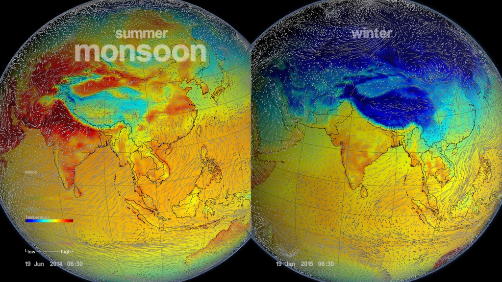
Monsoons: Wet, Dry, Repeat...
Go to this pageThis visualization shows the Asian monsoon and how it develops using observational and modeled data. It also showns some of the impacts.This video is also available on our YouTube channel. || monsoon_final_HD01.02500_print.jpg (1024x576) [182.2 KB] || final (1920x1080) [1.0 MB] || Monsoon_narrated_19201080p30.webm (1920x1080) [29.6 MB] || Monsoon_narrated_640x360p30.m4v (640x360) [43.4 MB] || monsoon_final_HD01_640x360_noNarration.m4v (640x360) [37.2 MB] || 3840x2160_16x9_60p (3840x2160) [1.0 MB] || monsoonnarrfull.en_US.srt [4.9 KB] || monsoonnarrfull.en_US.vtt [4.9 KB] || Monsoon_narrated_19201080p30.mp4 (1920x1080) [512.5 MB] || Monsoon_narrated_1920x1080p60_prores.mov (1920x1080) [7.3 GB] || monsoon_final_1920x1080p60_noNarration.mp4 (1920x1080) [387.4 MB] || monsoon_final_4kp30_noNarration.mp4 (3840x2160) [1.2 GB] ||
- ID: 4391 Visualization
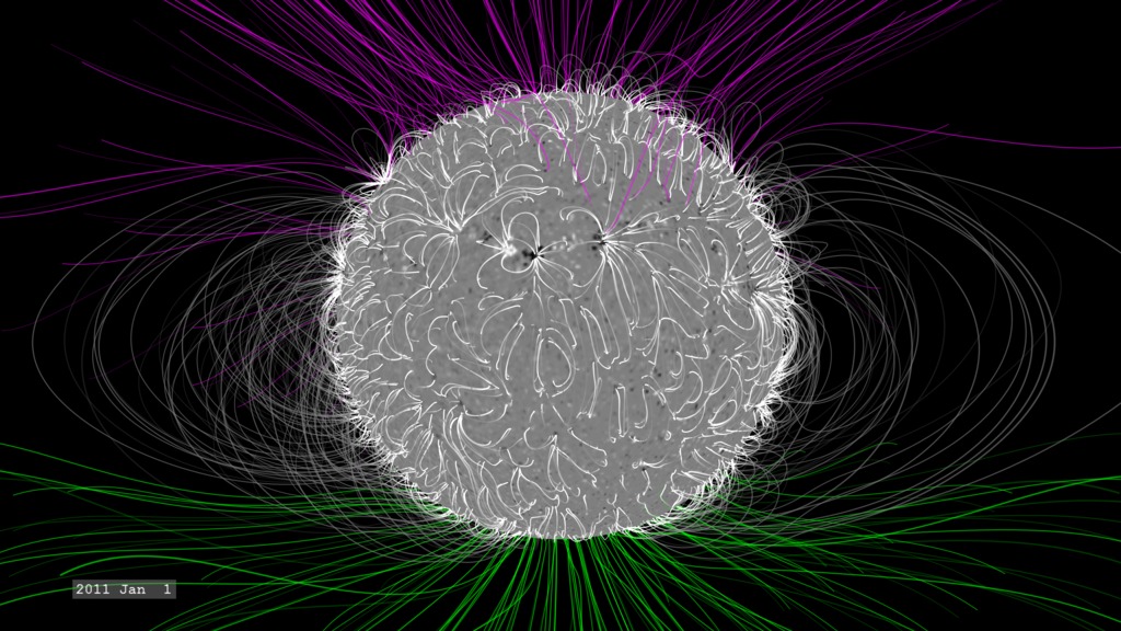
The Dynamic Solar Magnetic Field
Go to this pageA visualization of the slow changes of the solar magnetic field over the course of four years. || PFSSbasicView_inertial.HD1080i.0400_print.jpg (1024x576) [168.7 KB] || PFSSbasicView_inertial.HD1080i.0400_searchweb.png (180x320) [78.9 KB] || PFSSbasicView_inertial.HD1080i.0400_thm.png (80x40) [5.8 KB] || PFSSbasicView_inertial_1080p30.webm (1920x1080) [18.1 MB] || PFSSbasicView (1920x1080) [128.0 KB] || PFSSbasicView_inertial_1080p30.mp4 (1920x1080) [326.6 MB] || PFSSbasicView_inertial_1080p10.mp4 (1920x1080) [470.2 MB] || PFSSbasicView_HD1080p10.mov (1920x1080) [804.4 MB] || PFSSbasicView_inertial_1080p30.mp4.hwshow [232 bytes] ||
Playing with Time and Space
Visualizations where scales of time and space are changed to bring out hidden relationships.
- ID: 4565 Visualization
Seasonal Changes in Carbon Dioxide
Go to this pageNarrated visualization showing seasonal drawdown in carbon dioxideThis video is also available on our YouTube channel. || co2_science_comp.0740_print.jpg (1024x576) [118.8 KB] || co2_science_comp.0740_searchweb.png (180x320) [75.9 KB] || co2_science_comp.0740_thm.png (80x40) [6.1 KB] || CO2_Science_001_DDMMYY.m4v (1280x720) [66.6 MB] || CO2_Science_001_DDMMYY.webmhd.webm (1080x606) [17.7 MB] || CO2_Science_001_MM.m4v (1280x720) [66.5 MB] || comp (1920x1080) [0 Item(s)] || CO2_Science_001_DDMMYY.mp4 (1920x1080) [147.8 MB] || CO2_Science_001_MM.mp4 (1920x1080) [147.9 MB] || CO2_Science.en_US.srt [1.7 KB] || CO2_Science.en_US.vtt [1.7 KB] || CO2_Science_001_DDMMYY.mov (1920x1080) [1.1 GB] || CO2_Science_001_MM.mov (1920x1080) [1.1 GB] ||
- ID: 3838 Visualization
Incredible Solar Flare, Prominence Eruption and CME Event (304 angstroms)
Go to this pageOn June 7, 2011, an M-2 flare occurred on the Sun which released a very large coronal mass ejection (CME). Much of the ejected material is much cooler (less than about 80,000K) and therefore appears dark against the brighter solar disk.Material which does not reach solar escape velocity can be seen falling back and striking the solar surface, sometimes triggering smaller events.This image sequence is captured at one minute intervals and designed to play synchronously with animations 3839 (171 Ångstroms), 3840 (211 Ångstroms) and 3841 (1700 Ångstroms). ||
- ID: 4375 Visualization
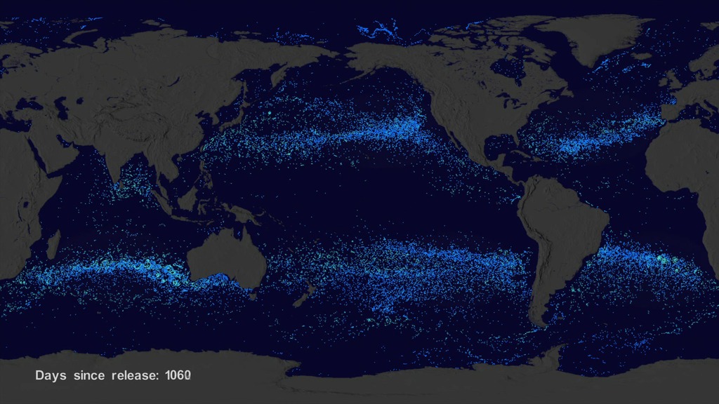
Garbage Patch Visualization Experiment
Go to this pageThis gallery was created for Earth Science Week 2015 and beyond. It includes a quick start guide for educators and first-hand stories (blogs) for learners of all ages by NASA visualizers, scientists and educators. We hope that your understanding and use of NASA's visualizations will only increase as your appreciation grows for the beauty of the science they portray, and the communicative power they hold. Read all the blogs and find educational resources for all ages at: the Earth Science Week 2015 page.You may have heard of "ocean garbage patches," areas in the ocean where litter and debris concentrates. This might stir up a vivid image of large blanketed areas of trash on the ocean surface that are easy to spot. But that’s not the case. Much of the debris consists of smaller pieces of plastic that are always moving and changing with the ocean currents, waves and winds. These can be difficult to see and predict. We set out to explore the processes and interactions that cause debris to flow to these patches using buoy and model data, and created a visualization based on our results. ||
- ID: 12412 Produced Video
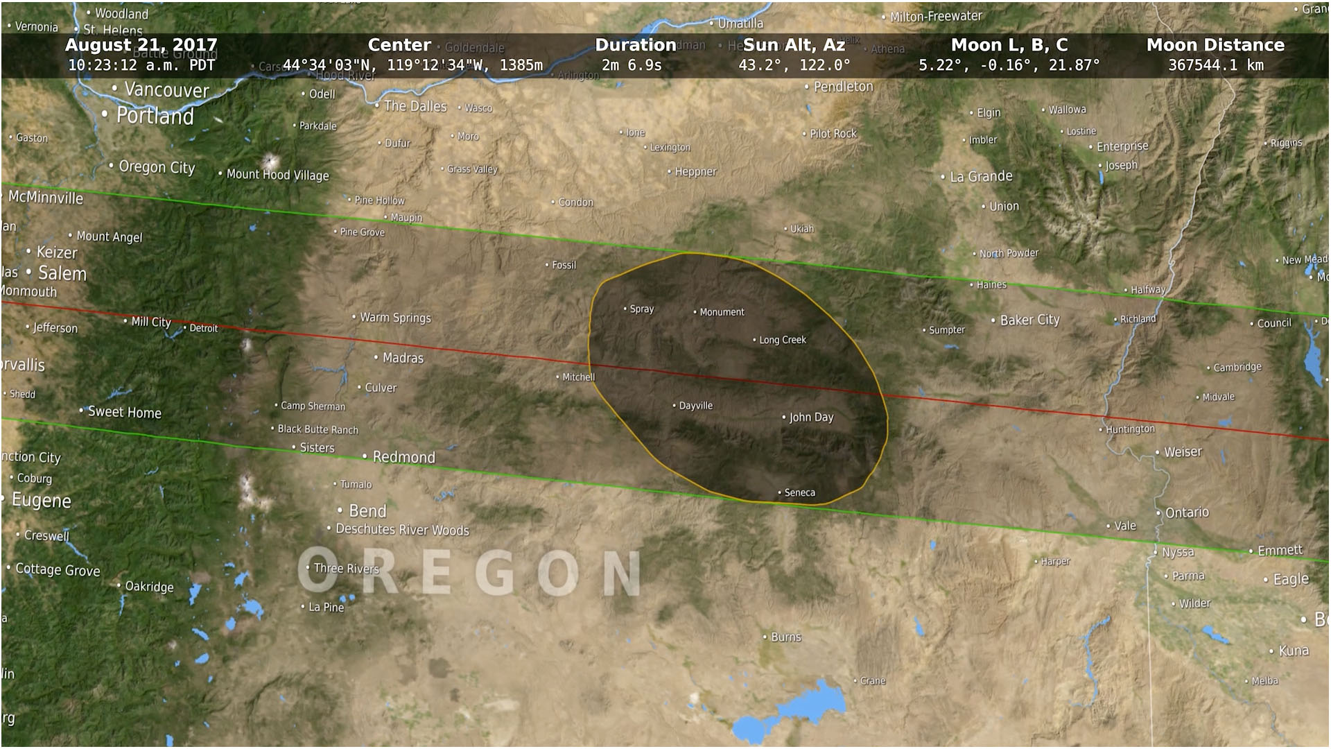
Tracing the 2017 Solar Eclipse
Go to this pageWhen depicting an eclipse path, data visualizers have usually chosen to represent the moon's shadow as an oval. By bringing in a variety of NASA data sets, visualizer Ernie Wright has created a new and more accurate representation of the eclipse. For the first time, we are able to see that the moon's shadow is better represented as a polygon. This more complicated shape is based NASA's Lunar Reconnaissance Orbiter's view of the mountains and valleys that form the moon's jagged edge. By combining moon's terrain, heights of land forms on Earth, and the angle of the sun, Wright is able to show the eclipse path with the greatest accuracy to date. ||
- ID: 3595 Visualization
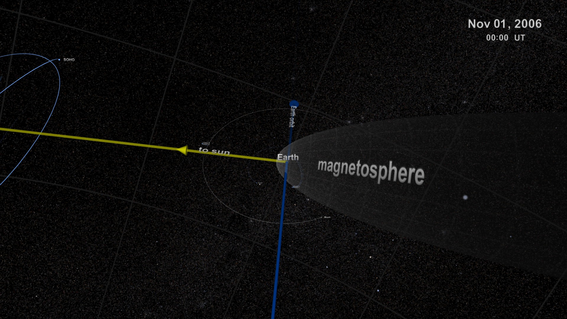
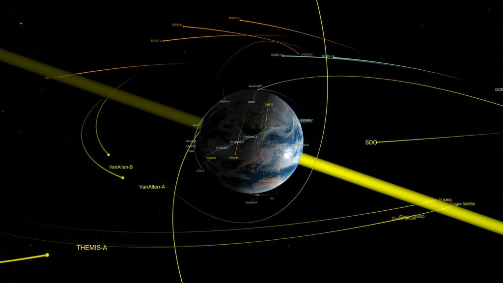
Sentinels of the Heliosphere
Go to this pageHeliophysics is a term to describe the study of the Sun, its atmosphere or the heliosphere, and the planets within it as a system. As a result, it encompasses the study of planetary atmospheres and their magnetic environment, or magnetospheres. These environments are important in the study of space weather.As a society dependent on technology, both in everyday life, and as part of our economic growth, space weather becomes increasingly important. Changes in space weather, either by solar events or geomagnetic events, can disrupt and even damage power grids and satellite communications. Space weather events can also generate x-rays and gamma-rays, as well as particle radiations, that can jeopardize the lives of astronauts living and working in space.This visualization tours the regions of near-Earth orbit; the Earth's magnetosphere, sometimes called geospace; the region between the Earth and the Sun; and finally out beyond Pluto, where Voyager 1 and 2 are exploring the boundary between the Sun and the rest of our Milky Way galaxy. Along the way, we see these regions patrolled by a fleet of satellites that make up NASA's Heliophysics Observatory Telescopes. Many of these spacecraft do not take images in the conventional sense but record fields, particle energies and fluxes in situ. Many of these missions are operated in conjunction with international partners, such as the European Space Agency (ESA) and the Japanese Space Agency (JAXA).The Earth and distances are to scale. Larger objects are used to represent the satellites and other planets for clarity.Here are the spacecraft featured in this movie:Near-Earth Fleet:Hinode: Observes the Sun in multiple wavelengths up to x-rays. SVS pageRHESSI : Observes the Sun in x-rays and gamma-rays. SVS pageTRACE: Observes the Sun in visible and ultraviolet wavelengths. SVS pageTIMED: Studies the upper layers (40-110 miles up) of the Earth's atmosphere.FAST: Measures particles and fields in regions where aurora form.CINDI: Measures interactions of neutral and charged particles in the ionosphere. AIM: Images and measures noctilucent clouds. SVS pageGeospace Fleet:Geotail: Conducts measurements of electrons and ions in the Earth's magnetotail. Cluster: This is a group of four satellites which fly in formation to measure how particles and fields in the magnetosphere vary in space and time. SVS pageTHEMIS: This is a fleet of five satellites to study how magnetospheric instabilities produce substorms. SVS pageL1 Fleet: The L1 point is a Lagrange Point, a point between the Earth and the Sun where the gravitational pull is approximately equal. Spacecraft can orbit this location for continuous coverage of the Sun.SOHO: Studies the Sun with cameras and a multitude of other instruments. SVS pageACE: Measures the composition and characteristics of the solar wind. Wind: Measures particle flows and fields in the solar wind. Heliospheric FleetSTEREO-A and B: These two satellites observe the Sun, with imagers and particle detectors, off the Earth-Sun line, providing a 3-D view of solar activity. SVS pageHeliopause FleetVoyager 1 and 2: These spacecraft conducted the original 'Planetary Grand Tour' of the solar system in the 1970s and 1980s. They have now travelled further than any human-built spacecraft and are still returning measurements of the interplanetary medium. SVS pageThis enhanced, narrated visualization was shown at the SIGGRAPH 2009 Computer Animation Festival in New Orleans, LA in August 2009; an eariler version created for AGU was called NASA's Heliophysics Observatories Study the Sun and Geospace. ||
Putting Data in Its Place
Data often refers to place and time, which can be very specific or can span a large area or many years. Adding information which clarifies the location of the visualization in time and space can enhance the viewer's experience.
- ID: 4129 Visualization
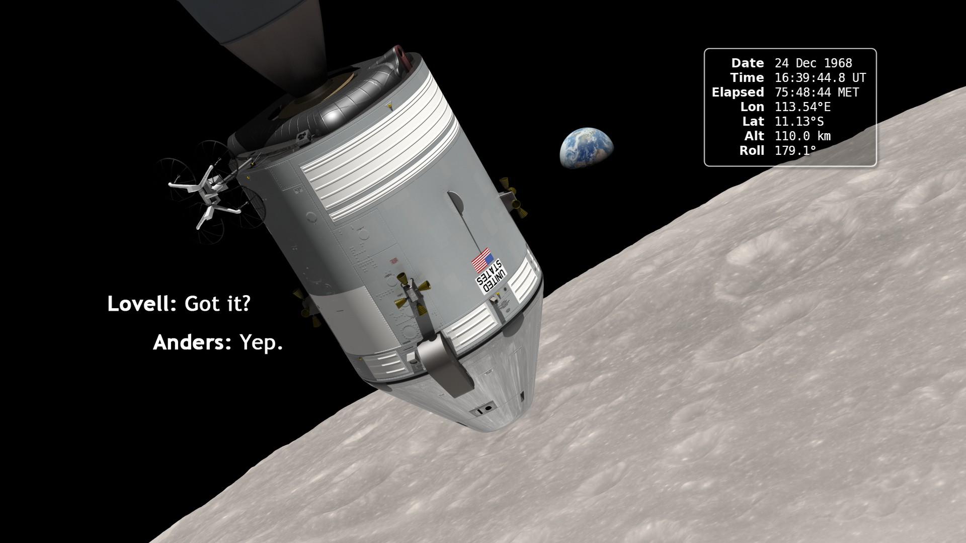
Earthrise: The 45th Anniversary
Go to this pageIn December of 1968, the crew of Apollo 8 became the first people to leave our home planet and travel to another body in space. But as crew members Frank Borman, James Lovell, and William Anders all later recalled, the most important thing they discovered was Earth.Using photo mosaics and elevation data from Lunar Reconnaissance Orbiter (LRO), this video commemorates the 45th anniversary of Apollo 8's historic flight by recreating the moment when the crew first saw and photographed the Earth rising from behind the Moon. Narrator Andrew Chaikin, author of A Man on the Moon, sets the scene for a three-minute visualization of the view from both inside and outside the spacecraft accompanied by the onboard audio of the astronauts.The visualization draws on numerous historical sources, including the actual cloud pattern on Earth from the ESSA-7 satellite and dozens of photographs taken by Apollo 8, and it reveals new, historically significant information about the Earthrise photographs. It has not been widely known, for example, that the spacecraft was rolling when the photos were taken, and that it was this roll that brought the Earth into view. The visualization establishes the precise timing of the roll and, for the first time ever, identifies which window each photograph was taken from.The key to the new work is a set of vertical stereo photographs taken by a camera mounted in the Command Module's rendezvous window and pointing straight down onto the lunar surface. It automatically photographed the surface every 20 seconds. By registering each photograph to a model of the terrain based on LRO data, the orientation of the spacecraft can be precisely determined.Andrew Chaikin's article Who Took the Legendary Earthrise Photo From Apollo 8? appeared in the January, 2018 issue of Smithsonian magazine. It includes the story of the making of this visualization.A Google Hangout discussion of this visualization between Ernie Wright (creator of the visualization), Andrew Chaikin, John Keller (LRO project scientist), and Aries Keck (NASA media specialist) was held on December 20, 2013. A replay of that hangout is available here.Ernie Wright presented a talk about the making of this animation at the 2014 SIGGRAPH Conference in Vancouver. He also wrote a NASA Wavelength blog entry about Earthrise that includes links to educator resources related to LRO. ||
- ID: 3619 Visualization
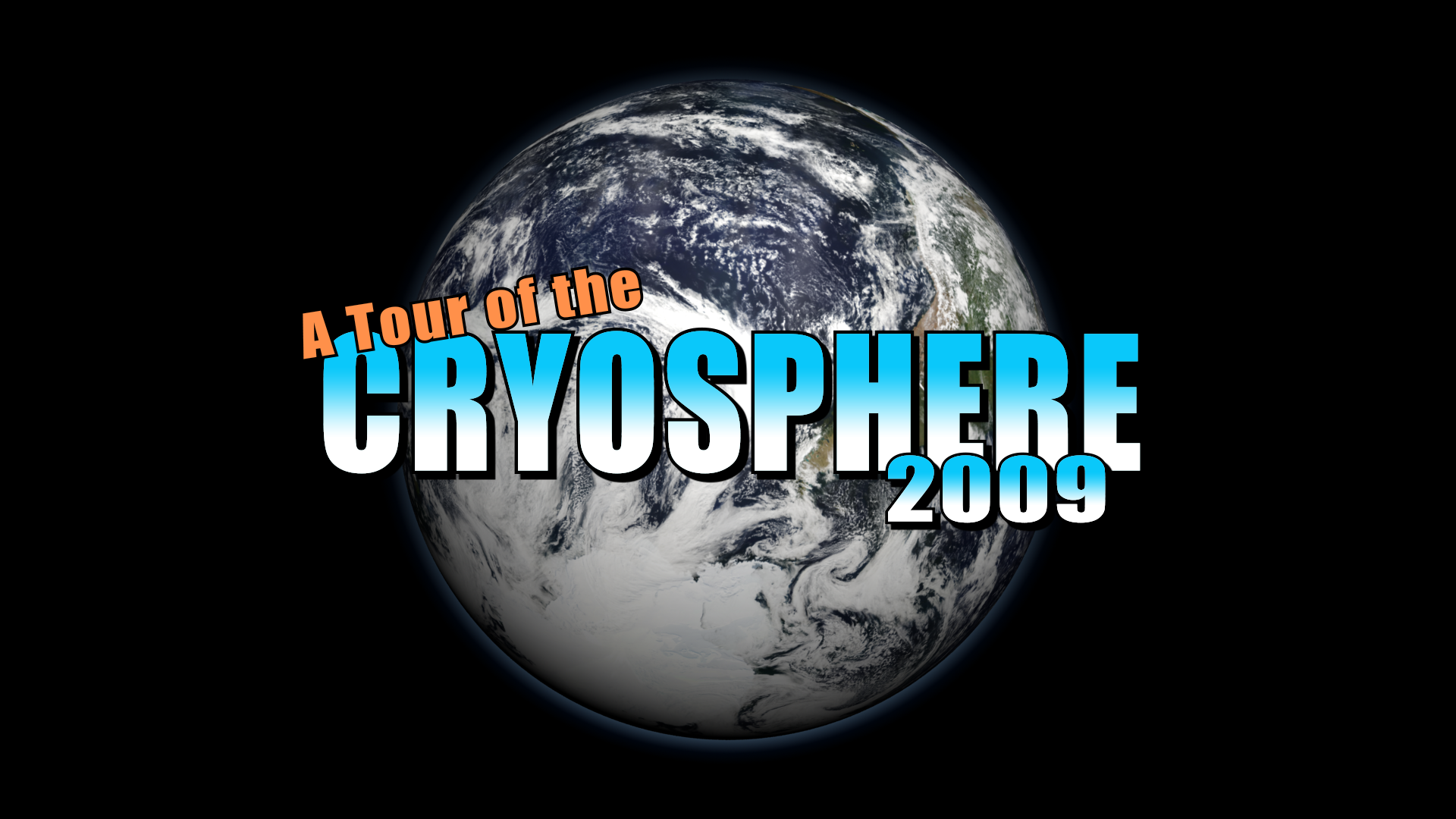
A Tour of the Cryosphere 2009
Go to this pageThe cryosphere consists of those parts of the Earth's surface where water is found in solid form, including areas of snow, sea ice, glaciers, permafrost, ice sheets, and icebergs. In these regions, surface temperatures remain below freezing for a portion of each year. Since ice and snow exist relatively close to their melting point, they frequently change from solid to liquid and back again due to fluctuations in surface temperature. Although direct measurements of the cryosphere can be difficult to obtain due to the remote locations of many of these areas, using satellite observations scientists monitor changes in the global and regional climate by observing how regions of the Earth's cryosphere shrink and expand.This animation portrays fluctuations in the cryosphere through observations collected from a variety of satellite-based sensors. The animation begins in Antarctica, showing some unique features of the Antarctic landscape found nowhere else on earth. Ice shelves, ice streams, glaciers, and the formation of massive icebergs can be seen clearly in the flyover of the Landsat Image Mosaic of Antarctica. A time series shows the movement of iceberg B15A, an iceberg 295 kilometers in length which broke off of the Ross Ice Shelf in 2000. Moving farther along the coastline, a time series of the Larsen ice shelf shows the collapse of over 3,200 square kilometers ice since January 2002. As we depart from the Antarctic, we see the seasonal change of sea ice and how it nearly doubles the apparent area of the continent during the winter.From Antarctica, the animation travels over South America showing glacier locations on this mostly tropical continent. We then move further north to observe daily changes in snow cover over the North American continent. The clouds show winter storms moving across the United States and Canada, leaving trails of snow cover behind. In a close-up view of the western US, we compare the difference in land cover between two years: 2003 when the region received a normal amount of snow and 2002 when little snow was accumulated. The difference in the surrounding vegetation due to the lack of spring melt water from the mountain snow pack is evident.As the animation moves from the western US to the Arctic region, the areas affected by permafrost are visible. As time marches forward from March to September, the daily snow and sea ice recede and reveal the vast areas of permafrost surrounding the Arctic Ocean.The animation shows a one-year cycle of Arctic sea ice followed by the mean September minimum sea ice for each year from 1979 through 2008. The superimposed graph of the area of Arctic sea ice at this minimum clearly shows the dramatic decrease in Artic sea ice over the last few years.While moving from the Arctic to Greenland, the animation shows the constant motion of the Arctic polar ice using daily measures of sea ice activity. Sea ice flows from the Arctic into Baffin Bay as the seasonal ice expands southward. As we draw close to the Greenland coast, the animation shows the recent changes in the Jakobshavn glacier. Although Jakobshavn receded only slightly from 1964 to 2001, the animation shows significant recession from 2001 through 2009. As the animation pulls out from Jakobshavn, the effect of the increased flow rate of Greenland costal glaciers is shown by the thinning ice shelf regions near the Greenland coast.This animation shows a wealth of data collected from satellite observations of the cryosphere and the impact that recent cryospheric changes are making on our planet.For more information on the data sets used in this visualization, visit NASA's EOS DAAC website.Note: This animation is an update of the animation 'A Short Tour of the Cryosphere', which is itself an abridged version of the animation 'A Tour of the Cryosphere'. The popularity of the earlier animations and their continuing relevance prompted us to update the datasets in parts of the animation and to remake it in high definition. In certain cases, our experiences in using the earlier work have led us to tweak the presentation of some of the material to make it clearer. Our thanks to Dr. Robert Bindschadler for suggesting and supporting this remake. ||
- ID: 4370 Visualization
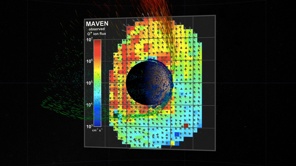
Solar Wind Strips the Martian Atmosphere
Go to this pageScientists have long suspected the solar wind of stripping the Martian upper atmosphere into space, turning Mars from a blue world to a red one. Now, NASA's MAVEN orbiter is observing this process in action, providing significant data on solar wind erosion at Mars.Watch this video on the NASA Goddard YouTube channel.Complete transcript available.This video is also available on our YouTube channel. || MarsAtmoLossExplainPreview.jpg (1920x1080) [993.6 KB] || APPLE_TV_4370_MAVEN_Mars_Atmo_Loss_appletv_subtitles.m4v (1280x720) [53.7 MB] || WEBM_4370_MAVEN_Mars_Atmo_Loss_APR.webm (960x540) [44.7 MB] || 4370_MAVEN_Mars_Atmo_Loss_appletv.m4v (1280x720) [53.7 MB] || NASA_TV_4370_MAVEN_Mars_Atmo_Loss.mpeg (1280x720) [369.5 MB] || 4370_MAVEN_Mars_Atmo_Loss_APR_Output.en_US.srt [2.3 KB] || 4370_MAVEN_Mars_Atmo_Loss_APR_Output.en_US.vtt [2.3 KB] || LARGE_MP4_4370_MAVEN_Mars_Atmo_Loss_large.mp4 (3840x2160) [111.3 MB] || YOUTUBE_HQ_4370_MAVEN_Mars_Atmo_Loss_youtube_hq.mov (3840x2160) [2.2 GB] || 4370_MAVEN_Mars_Atmo_Loss_APR.mov (3840x2160) [5.9 GB] ||
- ID: 4013 Visualization
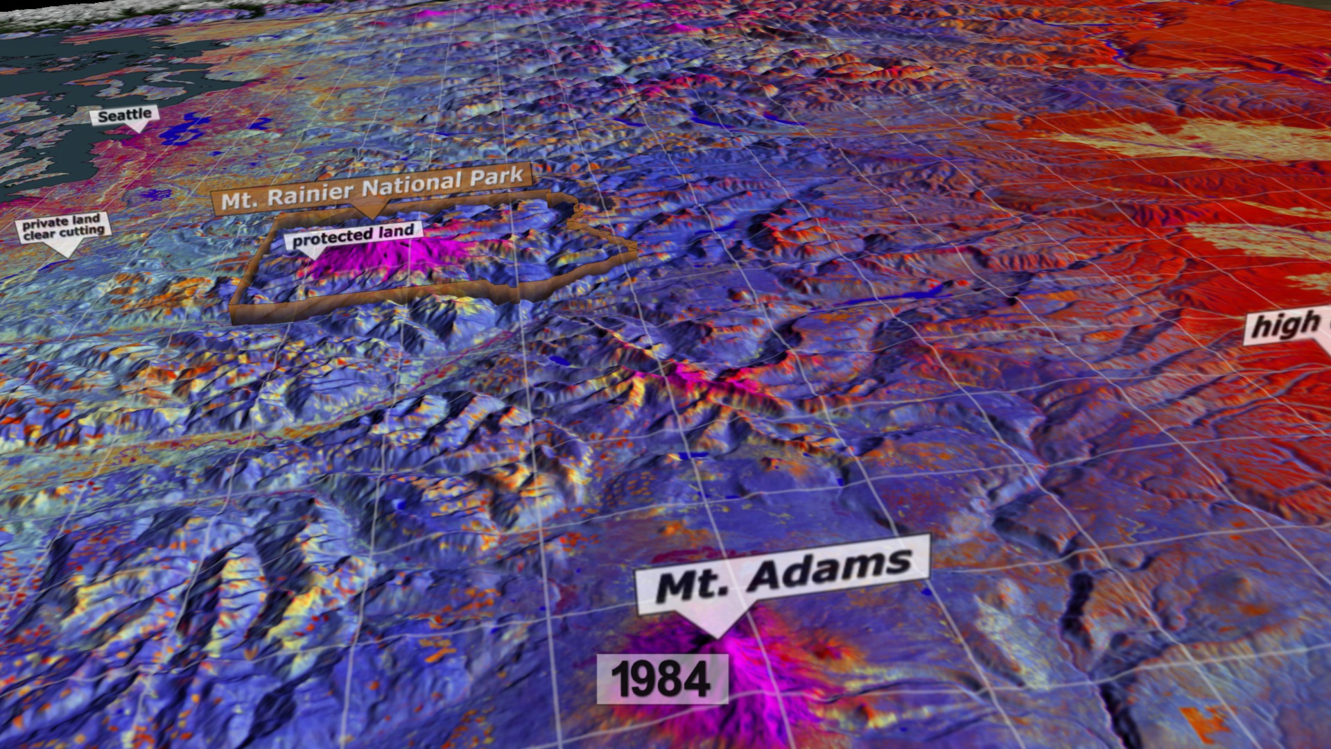
Life Histories from Landsat: 25 Years in the Pacific Northwest Forest
Go to this pageThis visualization shows a sequence of Landsat-based data in the Pacific Northwest. There is one data set for each year representing an aggregate of the approximate peak of the growing season (around August). The data was created using a sophisticated algorithm called LandTrendr. LandTrendr analyzes 'stacks' of Landsat scenes, looking for statistical trends in the data and filtering out noise. The algorithm evaluated data from more than 1,800 Landsat Thematic Mapper images, nearly 1 Terabyte of raw imagery, to define the life histories of each of more than 336 million pixels on the landscape. The resulting trends identify periods of stability and change that are displayed as colors.In these false color images, the colors represent types of land; for example, blue areas are forests; orange/yellow areas are agriculture; and, purple areas are urban. Each 'stack' is representative of a Landsat scene. There are 22 stacks stitched together to cover most of the U.S. Pacific Northwest. This processed data is used for science, natural resource management, and education.The visualization zooms into the Portland area showing different types of land such as agricultural, urban, and forests. We move south to a region that was evergreen forest for a number of years (blue), then was clear cut in 1999 (orange), then began to regrow (yellow). A graph shows the trajectories for a particular location in the clearcut as the years repeat. The dots represent the original data from Landsat; and, the line represents LandTrendr analysis. We move over to the Three Sisters region to show an area of pine forest that becomes infested with bark beetles in 2004. Next, we move to the southern foothills of Mount Hood where a budworm infestation is in progress; around 1991, the worms move on to another area and shrubs start to regrow. Next wemove to the east side of Mount Rainier National Park to see another budworm outbreak followed by shrub regrowth. Finally, we move to the west of Mount Rainier where we can see widespread clear cutting outside of the park, but no clear cutting inside the protected park land.Don't miss this related tour of the region. ||
- ID: 4315 Visualization
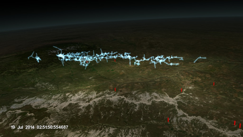
Lightning Over South Dakota
Go to this pageThe South Dakota Lightning Mapping Array (LMA) consists of 10 sensor stations that monitor very high frequency radio waves emitted by lightning. This dataset provides detailed information about a lightning event that occurred in western South Dakota around 2:50 PM on July 19th, 2014. The lightning flash contour data were generated by the scientists based on the raw LMA data. The lightning showed in this work lasts about 1.5 seconds. The animation repeats the lightning event 14 times played at the actual speed of the event to illustrate detailed 3D lightning observations and the lightning's dynamic progression providing a unique perspective on extreme weather. ||
From the Mind of the Scientist
Even in the absence of data, knowledge and imagination can combine to simulate reality and promote understanding.
- ID: 20252 Animation
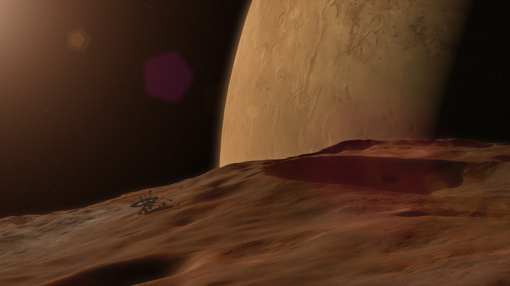
Phobos Electric Charging
Go to this pageThe interaction of the solar wind with the Martian moon Phobos creates a complex electrical environment that could impact future exploration. Complete transcript available.Watch this video on the NASA Goddard YouTube channel.Music provided by Killer Tracks: "Innovations" by Pascal Lengagne || PhobosChargingPreview.jpg (3840x2160) [1.6 MB] || PhobosChargingPreview_print.jpg (1024x576) [193.8 KB] || PhobosChargingPreview_searchweb.png (320x180) [95.8 KB] || PhobosChargingPreview_thm.png (80x40) [7.2 KB] || TWITTER_720-20252_Phobos_Electric_Charging_APR_twitter_720.mp4 (1280x720) [34.1 MB] || WEBM-20252_Phobos_Electric_Charging_APR.webm (960x540) [59.7 MB] || FACEBOOK_720-20252_Phobos_Electric_Charging_APR_facebook_720.mp4 (1280x720) [196.8 MB] || 20252_Phobos_Electric_Charging_APR_Output.en_US.srt [3.0 KB] || 20252_Phobos_Electric_Charging_APR_Output.en_US.vtt [3.0 KB] || YOUTUBE_4K-20252_Phobos_Electric_Charging_APR_youtube_4k.mp4 (3840x2160) [644.3 MB] || 20252_Phobos_Electric_Charging_APR.mov (3840x2160) [12.8 GB] ||
- ID: 20228 Animation
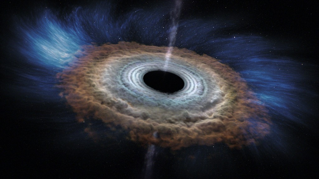
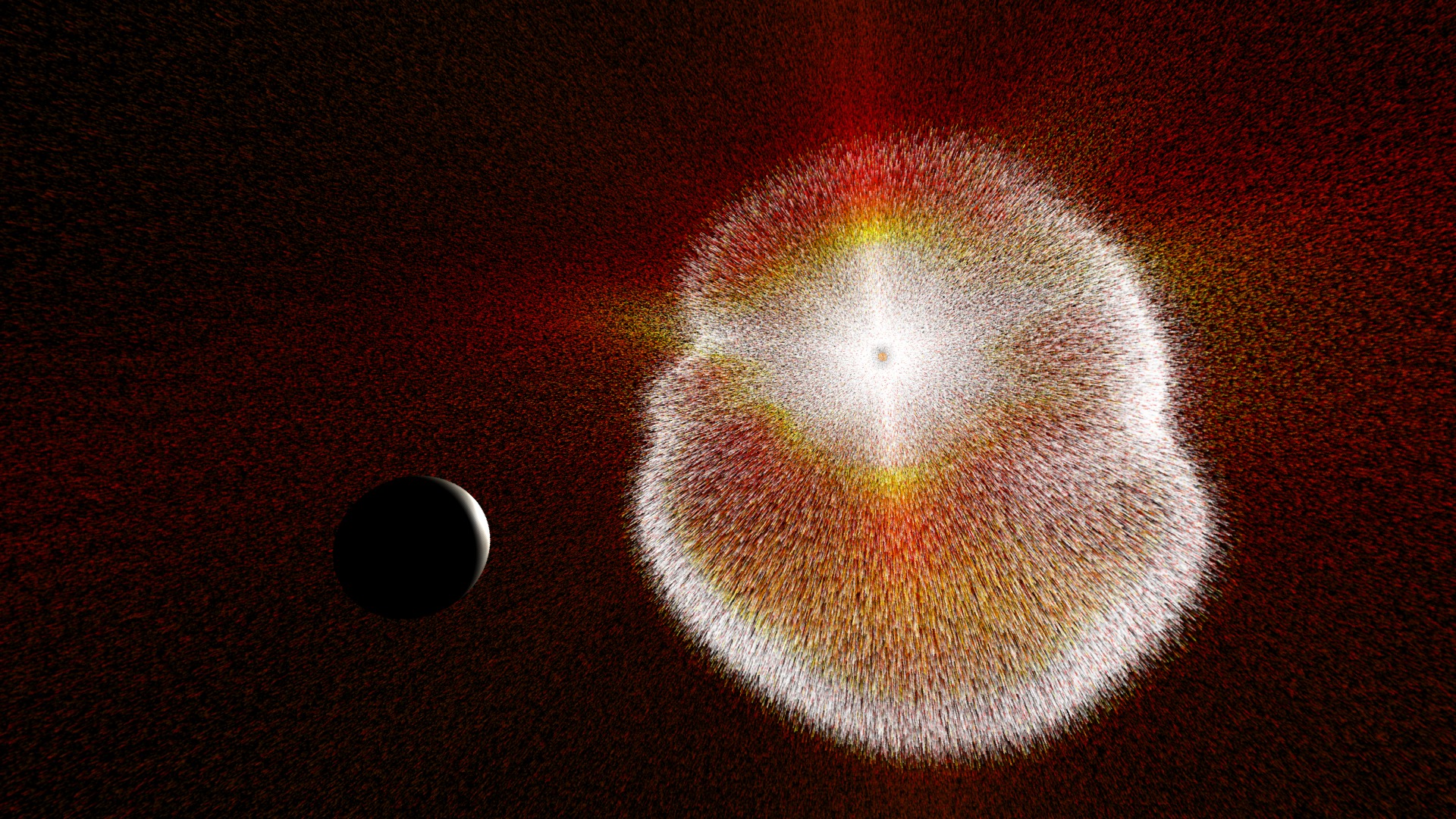
Massive Black Hole Shreds Passing Star (Animation Only)
Go to this pageA star approaching too close to a massive black hole is torn apart by tidal forces, as shown in this artist's rendering. Filaments containing much of the star's mass fall toward the black hole. Eventually these gaseous filaments merge into a smooth, hot disc glowing brightly in X-rays. As the disk forms, it's central region heats up tremendously, which drives a flow of material, called a wind, away from the disk.Credit: NASA's Goddard Space Flight Center/CI LabWatch this video on the NASA Goddard YouTube channel.For complete transcript, click here. || BlackHoleAnimation.1675_print.jpg (1024x576) [119.5 KB] || BlackHoleAnimation.1675_searchweb.png (320x180) [88.0 KB] || BlackHoleAnimation.1675_thm.png (80x40) [5.9 KB] || 20228_Swift_Tidal_ProRes_1920x1080_5994.webm (1920x1080) [4.8 MB] || 1920x1080_16x9_60p (1920x1080) [256.0 KB] || 20228_Swift_Tidal_ProRes_1920x1080_5994.mov (1920x1080) [1.4 GB] || 20228_Swift_Tidal_H264_1920x1080_5994.mov (1920x1080) [813.8 MB] ||
- ID: 20248 Animation
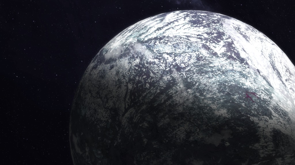
Generic Exoplanet Animations
Go to this pageAnimation imagining what an ice-covered exoplanet might look like. || Icy_Exoplanet_Still_print.jpg (1024x576) [144.3 KB] || Icy_Exoplanet_Still.png (3840x2160) [7.6 MB] || Icy_Exoplanet_Still_searchweb.png (320x180) [89.2 KB] || Icy_Exoplanet_Still_thm.png (80x40) [6.2 KB] || Icy_Exoplanet_H264_1080p.mov (1920x1080) [30.1 MB] || Icy_Exoplanet_H264_1080p.webm (1920x1080) [1.9 MB] || Icy (3840x2160) [0 Item(s)] || Icy_Exoplanet_H264_4K.mov (3840x2160) [39.4 MB] || Icy_Exoplanet_4k_ProRes.mov (3840x2160) [2.2 GB] ||
- ID: 20184 Animation
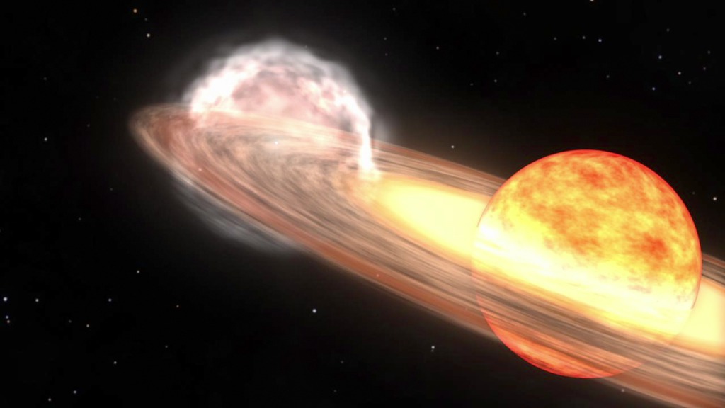
Fermi Sees a Nova
Go to this pageNASA's Fermi Gamma-ray Space Telescope has detected gamma-rays from a nova for the first time. The finding stunned observers and theorists alike because it overturns a long-standing notion that novae explosions lack the power for such high-energy emissions. In March, Fermi's Large Area Telescope (LAT) detected gamma rays — the most energetic form of light - from the nova for 15 days. Scientists believe that the emission arose as a million-mile-per-hour shock wave raced from the site of the explosion. A nova is a sudden, short-lived brightening of an otherwise inconspicuous star. The outburst occurs when a white dwarf in a binary system erupts in an enormous thermonuclear explosion. "In human terms, this was an immensely powerful eruption, equivalent to about 1,000 times the energy emitted by the sun every year," said Elizabeth Hays, a Fermi deputy project scientist at NASA's Goddard Space Flight Center in Greenbelt, Md. "But compared to other cosmic events Fermi sees, it was quite modest. We're amazed that Fermi detected it so strongly." More information here. ||
- ID: 20246 Animation
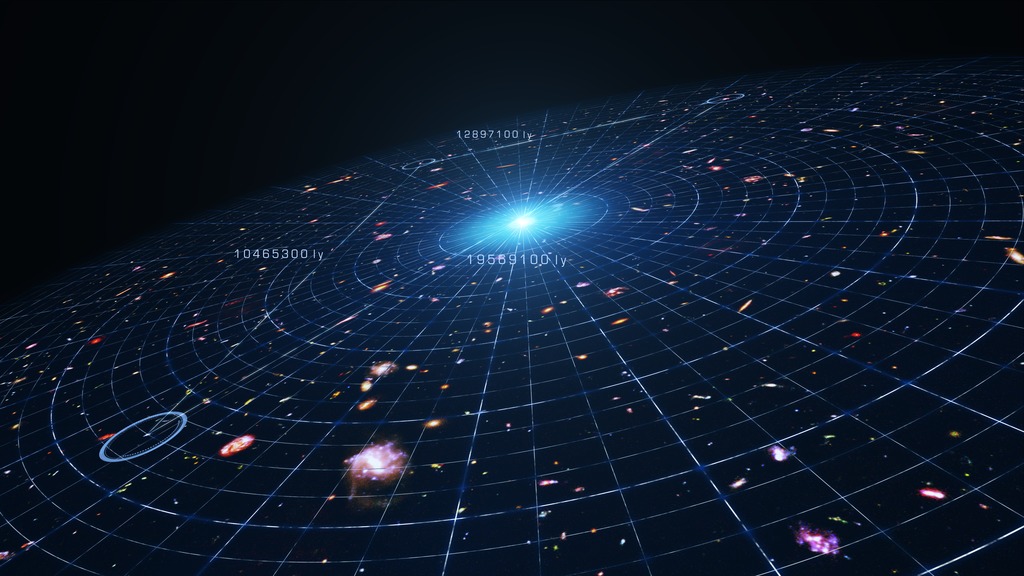
Dark Energy Expansion
Go to this pageAnimation illustrating the accelerating expansion of the universe. || WFirstExpansion_00599_print.jpg (1024x576) [151.6 KB] || WFirstExpansion_00599.png (3840x2160) [25.8 MB] || WFirstExpansion_00599_searchweb.png (320x180) [82.7 KB] || WFirstExpansion_00599_thm.png (80x40) [5.7 KB] || WFIRST_Dark_Energy_Expansion_H264_1080p.mov (1920x1078) [26.9 MB] || WFIRST_Dark_Energy_Expansion_H264_1080p.webm (1920x1078) [1.7 MB] || WFIRST_Dark_Energy_Expansion_4k_ProRes.mov (4104x2304) [768.2 MB] || 3840x2160_16x9_30p (4104x2304) [16.0 KB] || WFIRST_Dark_Energy_Expansion_H264_4K.mov (4096x2300) [36.0 MB] ||