Renderman Challenge
Overview
Scientific Visualization Studio assets for the 2022 RenderMan Challenge. For more 3D assets from NASA please visit the NASA 3D Resources page.
3D Assets
- ID: 4720 Visualization

CGI Moon Kit
Go to this pageThese color and elevation maps are designed for use in 3D rendering software. They are created from data assembled by the Lunar Reconnaissance Orbiter camera and laser altimeter instrument teams.
- ID: 4851 Visualization
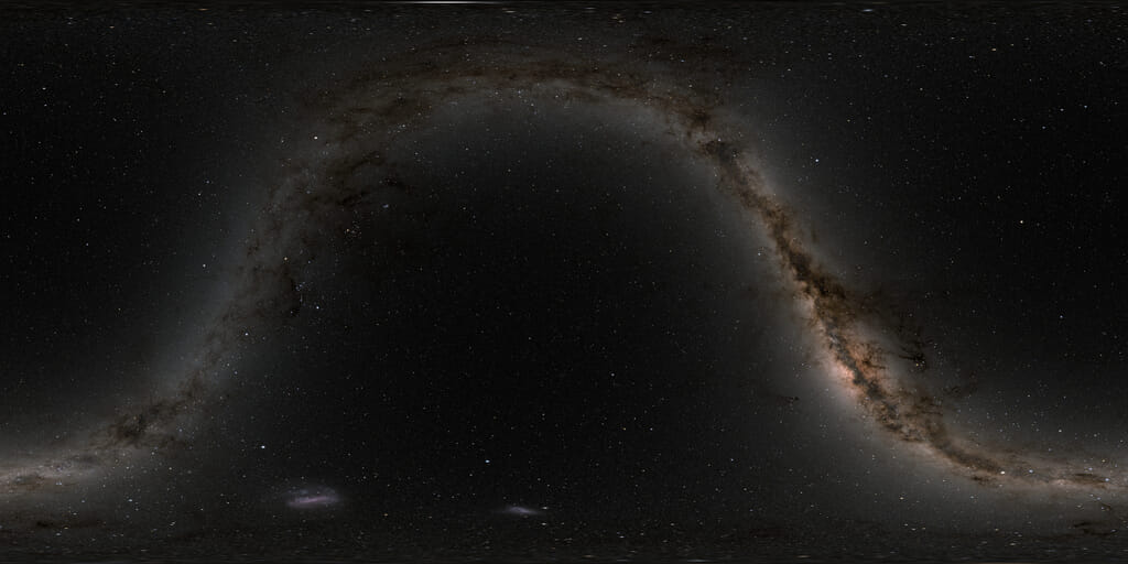
Deep Star Maps 2020
Go to this pageThe star map in celestial coordinates, at five different resolutions. The map is centered at 0h right ascension, and r.a. increases to the left. || starmap_2020_4k_print.jpg (1024x512) [41.8 KB] || starmap_2020_4k_searchweb.png (320x180) [53.9 KB] || starmap_2020_4k_thm.png (80x40) [5.5 KB] || starmap_2020_4k.exr (4096x2048) [34.3 MB] || starmap_2020_8k.exr (8192x4096) [124.5 MB] || starmap_2020_16k.exr (16384x8192) [422.9 MB] || starmap_2020_32k.exr (32768x16384) [1.4 GB] || starmap_2020_64k.exr (65536x32768) [3.8 GB] ||
- ID: 4439 Visualization
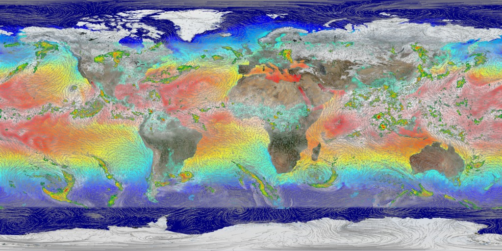
High Resolution Layers from "Monsoons: Wet, Dry, Repeat..."
Go to this pageComposited layers - all layers on || comp_4098x2048.09000_print.jpg (1024x512) [242.1 KB] || comp_4098x2048.01000_searchweb.png (180x320) [127.2 KB] || comp_1920x1080p30.webm (1920x1080) [47.8 MB] || comp (4096x2048) [0 Item(s)] || comp_2048x1024p30.mp4 (2048x1024) [1.6 GB] || comp_1920x1080p30.mp4 (1920x1080) [1.6 GB] || comp_4098x2048_p30.mp4 (4096x2048) [6.4 GB] || comp_1920x1080p30.mp4.hwshow [183 bytes] ||