Cindy's Favorite Projects
3D Stereoscopic Visualizations
These visualizations are offered in two different modes in order to accomodate viewing in stereoscopic systems. Modes include the Left and Right Eye separate as well as Left and Right Eye side-by-side combined on the same frame.
- ID: 3783 Visualization
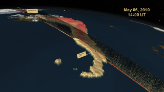
Iceland's Eyjafjallajökull Volcanic Ash Plume May 6-8, 2010 - Stereoscopic Version
Go to this pageDuring April and May, 2010, the Eyjafjallajökull volcano on Iceland's southern coast erupted, creating an expansive ash cloud that disrupted air traffic throughout Europe and across the Atlantic. This animation shows the flow of this ash cloud for three days in early May on an hourly basis as sensed from a geostationary satellite. The ash cloud heights were determined using an approach developed by NOAA/NESDIS/STAR for the next generation of Geostationary Operational Environmental Satellite (GOES-R). Data from EUMETSAT's Spinning Enhanced Visible and Infrared Imager (SEVIRI) was used as a proxy for GOES-R Advanced Baseline Imager (ABI) data. This data is shown intersecting with the CALIPSO Parallel Attenuated Backscatter curtain on May 6th. In this page the visualization content is offered in two different modes to accommodate stereoscopic systems as: Left and Right Eye separate and Left and Right Eye side-by-side combined on the same frame. ||
- ID: 3766 Visualization
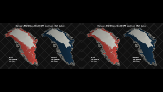
2007 Greenland Melt Season Study - Stereoscopic Version
Go to this pageThe Greenland ice sheet has been the focus of attention recently because of increasing melt in response to regional climate change. Several different remote sensing data products have been used to study surface and near-surface melt characteristics of the Greenland ice sheet for the 2007 melt season when record melt extent and runoff occurred. Here, MODIS daily land surface temperature and a special diurnal melt product, derived from QuikSCAT scatterometer data, measure the evolution of melt on the ice sheet. Although these daily products are sensitive to different geophysical features, they show excellent correspondence when surface melt is present. This animation displays these two geophysical data products of the Greenland ice sheet side-by-side, showing MODIS data on the left side and QuikSCAT data on the right. The 2007 melt season is shown twice. In the first sequence, MODIS surface temperature is compared with several categories of QuikSCAT melt between March 15th and October 13th, 2010. During this sequence, active melt detected by QuikSCAT is shown in light blue, reduced melt is medium blue, and completed melt is dark blue. For the MODIS, surface temperature is shown with the color scale — red indicates a surface temperature greater than -1 degree Celsius. As MODIS shows warmer surface temperature as the melt season progresses, QuikSCAT consistently identifies the corresponding melt.In the second sequence, the MODIS and QuikSCAT melted regions of the ice sheet were accumulated during the melt season. QuikSCAT captures melt earlier, and then melt is detected by MODIS shortly afterward at a higher spatial resolution. The final result (frame) shows the seasonal melt extent which was consistently delineated by both sensors. The cross-verification of these independent measurements, by two different instruments on different satellites, provides a higher confidence level in the melt observations, reducing the uncertainty in climate assessment of Greenland melt.This visualization is a stereoscopic version of animation entry: #3738: 2007 Greenland Melt Season Study. In this page the visualization content is offered in two different modes to accommodate stereoscopic systems, such as: Left and Right Eye separate and Left and Right Eye side-by-side combined on the same frame. ||
- ID: 3578 Visualization
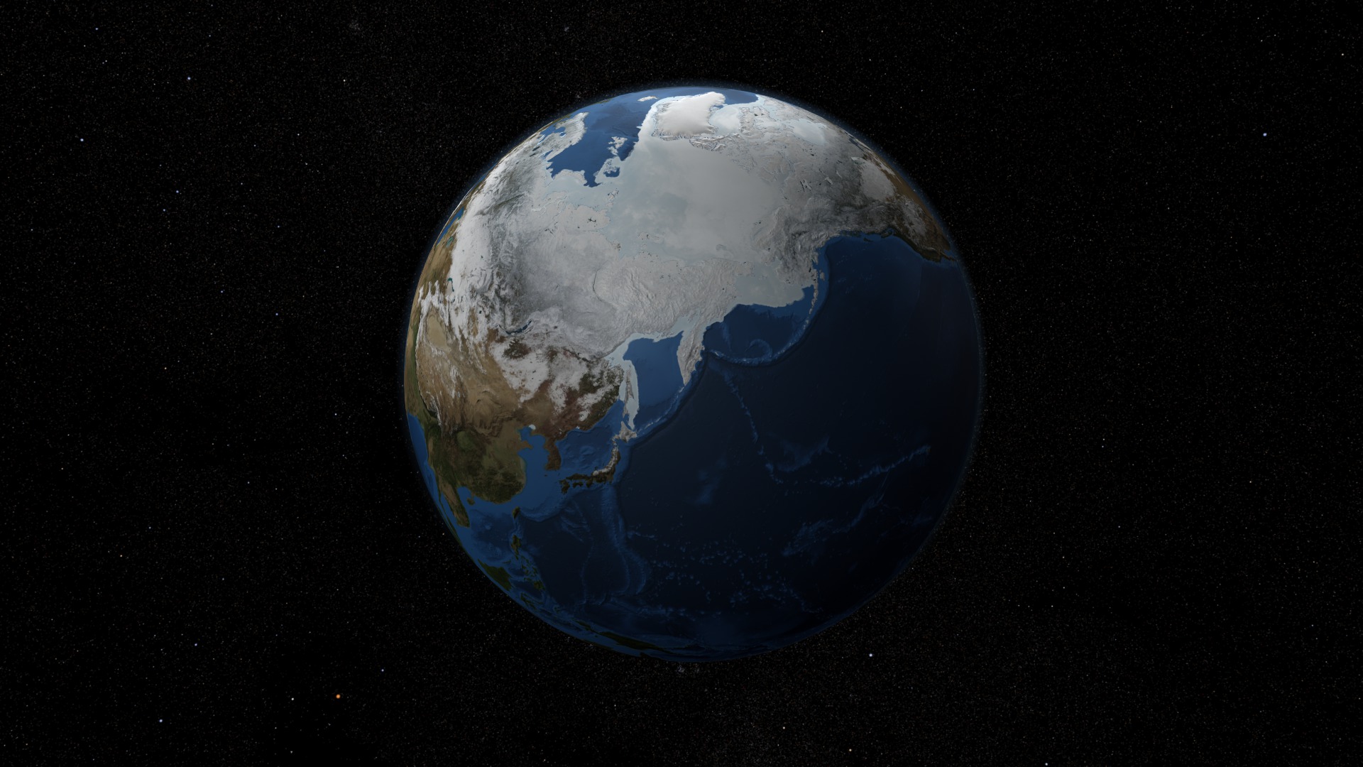
AMSR-E Arctic Sea Ice: 2005 to 2008 - Stereoscopic Version
Go to this pageSea ice is frozen seawater floating on the surface of the ocean. Some sea ice is semi-permanent, persisting from year to year, and some is seasonal, melting and refreezing from season to season. The sea ice cover reaches its minimum extent at the end of each summer and the remaining ice is called the perennial ice cover.In this animation, the globe slowly rotates one full rotation while the Arctic sea ice and seasonal land cover change throughout the years. The animation begins on September 21, 2005 when sea ice in the Arctic was at its minimum extent, and continues through September 20, 2008. This time period repeats twice during the animation, playing at a rate of one frame per day. Over the terrain, monthly data from the seasonal Blue Marble Next Generation fades slowly from month to month. Over the water, Arctic sea ice changes from day to day. This visualization is a stereoscopic version of animation entry: #3571: AMSR-E Arctic Sea Ice: 2005 to 2008In this page the visualization content is offered in two different modes to accomodate stereoscopic systems, such as: Left and Right Eye separate and Left and Right Eye side-by-side combined on the same frame. ||
Special Format Productions
- ID: 10403 Produced Video
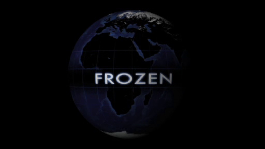
FROZEN: A Spherical Movie About the Cryosphere
Go to this pageNASA's home for spherical films on Magic Planet. Download the Magic Planet-ready movie file here.Released on March 27, 2009, FROZEN is NASA's second major production for the Science On a Sphere platform, a novel cinema-in-the-round technology developed by the Space Agency's sibling NOAA. Viewers see the Earth suspended in darkness as if it were floating in space. Moving across the planet's face, viewers see the undulating wisps of clouds, the ephemeral sweep of fallen snow, the churning crash of shifting ice, and more.FROZEN brings the Earth alive. Turning in space, the sphere becomes a portal onto a virtual planet, complete with churning, swirling depictions of huge natural forces moving below. FROZEN features the global cryosphere, those places on Earth where the temperature doesn't generally rise above water's freezing point. As one of the most directly observable climate gauges, the changing cryosphere serves as a proxy for larger themes.But just as thrilling as this unusual—and unusually realistic—look at the planet's structure and behavior is the sheer fun and fascination of looking at a spherically shaped movie. FROZEN bends the rules of cinema, revealing new ways to tell exciting, valuable stories of all kinds. The movie may be FROZEN, but the experience itself rockets along. ||
Productions with Narration
- ID: 3619 Visualization
A Tour of the Cryosphere 2009
Go to this pageThe cryosphere consists of those parts of the Earth's surface where water is found in solid form, including areas of snow, sea ice, glaciers, permafrost, ice sheets, and icebergs. In these regions, surface temperatures remain below freezing for a portion of each year. Since ice and snow exist relatively close to their melting point, they frequently change from solid to liquid and back again due to fluctuations in surface temperature. Although direct measurements of the cryosphere can be difficult to obtain due to the remote locations of many of these areas, using satellite observations scientists monitor changes in the global and regional climate by observing how regions of the Earth's cryosphere shrink and expand.This animation portrays fluctuations in the cryosphere through observations collected from a variety of satellite-based sensors. The animation begins in Antarctica, showing some unique features of the Antarctic landscape found nowhere else on earth. Ice shelves, ice streams, glaciers, and the formation of massive icebergs can be seen clearly in the flyover of the Landsat Image Mosaic of Antarctica. A time series shows the movement of iceberg B15A, an iceberg 295 kilometers in length which broke off of the Ross Ice Shelf in 2000. Moving farther along the coastline, a time series of the Larsen ice shelf shows the collapse of over 3,200 square kilometers ice since January 2002. As we depart from the Antarctic, we see the seasonal change of sea ice and how it nearly doubles the apparent area of the continent during the winter.From Antarctica, the animation travels over South America showing glacier locations on this mostly tropical continent. We then move further north to observe daily changes in snow cover over the North American continent. The clouds show winter storms moving across the United States and Canada, leaving trails of snow cover behind. In a close-up view of the western US, we compare the difference in land cover between two years: 2003 when the region received a normal amount of snow and 2002 when little snow was accumulated. The difference in the surrounding vegetation due to the lack of spring melt water from the mountain snow pack is evident.As the animation moves from the western US to the Arctic region, the areas affected by permafrost are visible. As time marches forward from March to September, the daily snow and sea ice recede and reveal the vast areas of permafrost surrounding the Arctic Ocean.The animation shows a one-year cycle of Arctic sea ice followed by the mean September minimum sea ice for each year from 1979 through 2008. The superimposed graph of the area of Arctic sea ice at this minimum clearly shows the dramatic decrease in Artic sea ice over the last few years.While moving from the Arctic to Greenland, the animation shows the constant motion of the Arctic polar ice using daily measures of sea ice activity. Sea ice flows from the Arctic into Baffin Bay as the seasonal ice expands southward. As we draw close to the Greenland coast, the animation shows the recent changes in the Jakobshavn glacier. Although Jakobshavn receded only slightly from 1964 to 2001, the animation shows significant recession from 2001 through 2009. As the animation pulls out from Jakobshavn, the effect of the increased flow rate of Greenland costal glaciers is shown by the thinning ice shelf regions near the Greenland coast.This animation shows a wealth of data collected from satellite observations of the cryosphere and the impact that recent cryospheric changes are making on our planet.For more information on the data sets used in this visualization, visit NASA's EOS DAAC website.Note: This animation is an update of the animation 'A Short Tour of the Cryosphere', which is itself an abridged version of the animation 'A Tour of the Cryosphere'. The popularity of the earlier animations and their continuing relevance prompted us to update the datasets in parts of the animation and to remake it in high definition. In certain cases, our experiences in using the earlier work have led us to tweak the presentation of some of the material to make it clearer. Our thanks to Dr. Robert Bindschadler for suggesting and supporting this remake. ||
- ID: 3180 Visualization
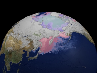
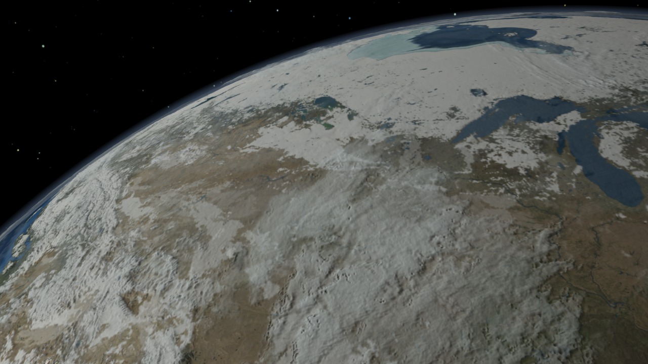
MODIS Daily Global Snow Cover and Sea Ice Surface Temperature as seen in the SIGGRAPH 2005 Electronic Theater
Go to this pageThis animation showing snow cover and sea ice surface temperature in the Northern Hemisphere portrays data collected from daily MODIS satellite images acquired during the winter of 2002-2003. Darkness increases with the onset of autumn, reaching a maximum at the Winter Solstice on December 21st. Thereafter, the circle of darkness shrinks as the period of daylight increases. Daily changes in sea ice are shown as ice surface temperature, which is related to the air temperature and the concentration of the sea ice. Sea ice surface temperatures range from about -40 to -2 degrees Celsius. Here, ice surface temperatures are depicted by colors, described by a color bar shown below. The snow tracks of several winter storms across the United States can be clearly seen. With an albedo of up to 80 percent or more, snow-covered terrain reflects most of the incoming solar radiation back into space, cooling the lower atmosphere. When snow cover melts, the albedo drops suddenly to less than about 30 percent, allowing the ground to absorb more solar radiation, heating the Earth's surface and lower atmosphere. Rapid changes in albedo, resultingfrom snowfall and snow melt, cause significant changes in the regional energy balance. This animation was accepted into the prestigious 2005 SIGGRAPH Electronic Theater, where it was shown during the annual conference from July 31 through August 4, 2005 in Los Angeles, CA. For more information on the data sets used in this visualization, visit NASA's EOS DAAC website. ||
- ID: 2707 Visualization

Multisensor Fire Observations
Go to this pageFrom space, we can understand fires in ways that are impossible from the ground. New Earth-observing satellites capture the significant impact of fires on our planet. In this animation of fires around the globe in 2002, each red dot marks a new fire. Dots change color to yellow after a few days and to black when fires burn out. From brush fires in Africa to forest fires in North America, satellites are locating every significant fire on Earth to within one kilometer. In the summer and fall burning seasons, particularly destructive fires occurred in Colorado, Arizona, and Oregon. ||
HD Data Animations
- ID: 3698 Visualization
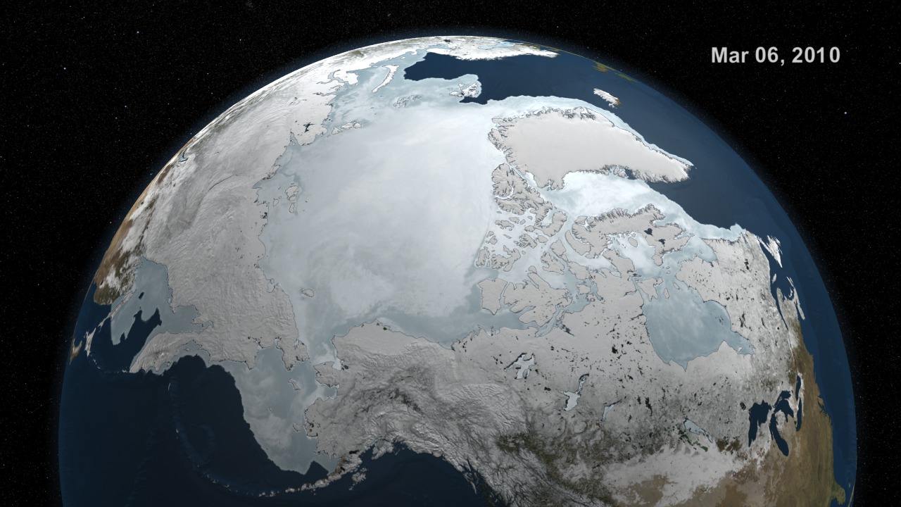
AMSR-E Arctic Sea Ice: September 2009 to March 2010
Go to this pageSea ice is frozen seawater floating on the surface of the ocean. Some sea ice is semi-permanent, persisting from year to year, and some is seasonal, melting and refreezing from season to season. The sea ice cover reaches its minimum extent at the end of each summer and the remaining ice is called the perennial ice cover.In this animation, the Arctic sea ice and seasonal land cover change progress through time, from September 1, 2009 when sea ice in the Arctic was near its minimum extent, through March 30, 2010. The animation plays at a rate of six frames per day or ten days per second. Over the water, Arctic sea ice changes from day to day showing a running 3-day maximum sea ice concentration in the region where the concentration is greater than 15%. The blueish white color of the sea ice is derived from a 3-day running maximum of the AMSR-E 89 GHz brightness temperature. Over the terrain, monthly data from the seasonal Blue Marble Next Generation fades slowly from month to month. ||
- ID: 3687 Visualization
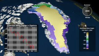
Greenland Ice Sheet Mass Changes from NASA GSFC GRACE Mascon Solutions with Banded Color Scale
Go to this pageLuthcke, S.B., D.D. Rowlands, J.J. McCarthy, A. Arendt, T. Sabaka, J.P. Boy, F.G. Lemoine, "Recent Changes of the Earth's Land Ice from GRACE, " presented at 2009 Fall AGU, H13G-02 (693337), Dec. 14, 2009.The mass changes of the Greenland Ice Sheet (GIS) are computed from the Gravity Recovery and Climate Experiment (GRACE) inter-satellite range-rate observations for the period April 5, 2003 - July 25, 2009. The mass of the GIS has been computed at 10-day intervals and 200km spatial resolution from a regional high-resolution mascon solution (Luthcke and others, 2008 and 2006). The animation shows the change in mass referenced from April 5, 2003. The spatial variation in surface mass is shown in centimeters equivalent height of water. The time variation of the GIS mass is shown in the x-y plot insert with units of Gigatons.Corresponding author:Scott B. LuthckeNASA GSFCPlanetary Geodynamics Laboratory, Code 698Scott.B.Luthcke@nasa.gov ||
- ID: 3648 Visualization
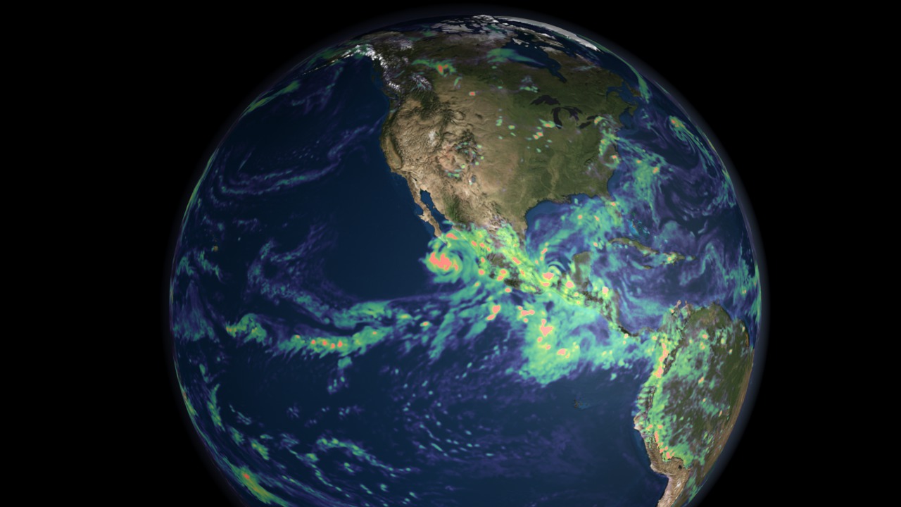
Components of the Water Cycle
Go to this pageWater regulates climate, storing heat during the day and releasing it at night. Water in the ocean and atmosphere carry heat from the tropics to the poles. The process by which water moves around the earth, from the ocean, to the atmosphere, to the land and back to the ocean is called the water cycle. The animations below each portray a component of the water cycle. All use an identical view and camera motion to allow for easy compositing.Data for the animation of global sea surface temperature was derived from a model run of ECCO's Ocean General Circulation Model. See http://www.ecco-group.org/model.htm for more information on ECCO.Data for the animation of atmospheric phenomena was created using data from the GEOS-5 atmospheric model on the cubed-sphere, run at 14-km global resolution for 25-days. Variables animated here include evaporation, water vapor and precipitation.For more information on the GEOS-5 see http://gmao.gsfc.nasa.gov/systems/geos5.For more information on the cubed-sphere work see http://science.gsfc.nasa.gov/610.3/cubedsphere.html.All three of these animations are time synchronous throughout the animation to allow cross fades during compositing.The final animation shown here, a pulsing network of rivers over the continents, represents the flow of water from land back into the ocean, thereby completing the water cycle.A flat version of these animations can be found in item #3811. ||
- ID: 3644 Visualization

Hourly Evaporation from the GEOS-5 Model
Go to this pageThis animation of the global hourly evaporation shows how heating from the sun during the day causes increased evaporation over land areas. Two versions of this animation are provided: one with a day/night clock inset and one without. The animation was created using data from the GEOS-5 atmospheric model on the cubed-sphere, run at 14-km global resolution for 30-days. For more information on the GEOS-5, see http://gmao.gsfc.nasa.gov/systems/geos5. For more information on the cubed-sphere work, see http://sivo.gsfc.nasa.gov/cubedsphere_overview.html. ||
- ID: 3643 Visualization

Hourly Atmospheric Water Vapor from the GEOS-5 Model
Go to this pageThese three animations portray the hourly flow of atmospheric water vapor around the world. The animations were created using data from the GEOS-5 atmospheric model on the cubed-sphere, run at 14-km global resolution for 30-days. For more information on the GEOS-5, see http://gmao.gsfc.nasa.gov/systems/geos5 . For more information on the cubed-sphere work, see http://sivo.gsfc.nasa.gov/cubedsphere_overview.html. ||
- ID: 3383 Visualization
Sequence of Clouds, Snow Cover, Sea Ice, Sea Surface Temperature and Biosphere
Go to this pageThis animation is part of an NSF-funded, international project, Exploring Time. The two-hour television special, broadcast on the Discovery Channel in the spring of 2007, explores how the world changes over different timescales ... from billionths of seconds to billions of years. This animation portrays a variety of remotely sensed data elements at different temporal resolutions.Initially, the animation shows cloud cover in motion over North America in half-hour increments from Nov. 26 to Dec. 7, 2005. The temporal pace quickens to show a 5-day moving average of daily MODIS snow cover along with daily AMSR-E sea ice from Dec. 7, 2005 to Mar. 15, 2006. As the view swings south over the Gulf of Mexico, the AMSR-E Sea Surface Temperature reveals warming ocean temperatures from March through August, 2006. As it passes over the Atlantic Ocean, the biosphere fades into view, showing both chlorophyll concentration in the ocean along with Normalized Difference Vegetation Index over the land areas. The biosphere animates over time while the view pans over northern Africa and Europe, showing data collected from September 2002 through February 2006.This program was also broadcast in Japan through a partnership with the NHK international broadcasting service and in France through a partnership with the ARTE television network. ||
Posters
- ID: 3670 Visualization
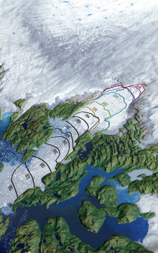
Poster of the Jakobshavn Glacier Calving Front Recession from 1851 to 2009
Go to this pageJakobshavn Isbrae is located on the west coast of Greenland at Latitude 69 N. The ice front, where the glacier calves into the sea, receded more than 40 km between 1850 and 2006. Between 1850 and 1964 the ice front retreated at a steady rate of about 0.3 km/yr, after which it occupied approximately the same location until 2001, when the ice front began to recede again, but far more rapidly at about 3 km/yr. As more ice moves from glaciers on land into the ocean, it causes a rise in sea level. Jakobshavn Isbrae is Greenland's largest outlet glacier, draining 6.5 percent of Greenland's ice sheet area. The ice stream's speed-up and near-doubling of the ice flow from land into the ocean has increased the rate of sea level rise by about .06 millimeters (about .002 inches) per year, or roughly 4 percent of the 20th century rate of sea level increase. This may be due in part to the numerous melt lakes visible here near the top of the image. These are believed to lubricate the layer between the ice sheet and bedrock, causing the ice to flow faster toward the sea. See an animation illustrating this acceleration in item #10153. ||
- ID: 3402 Visualization
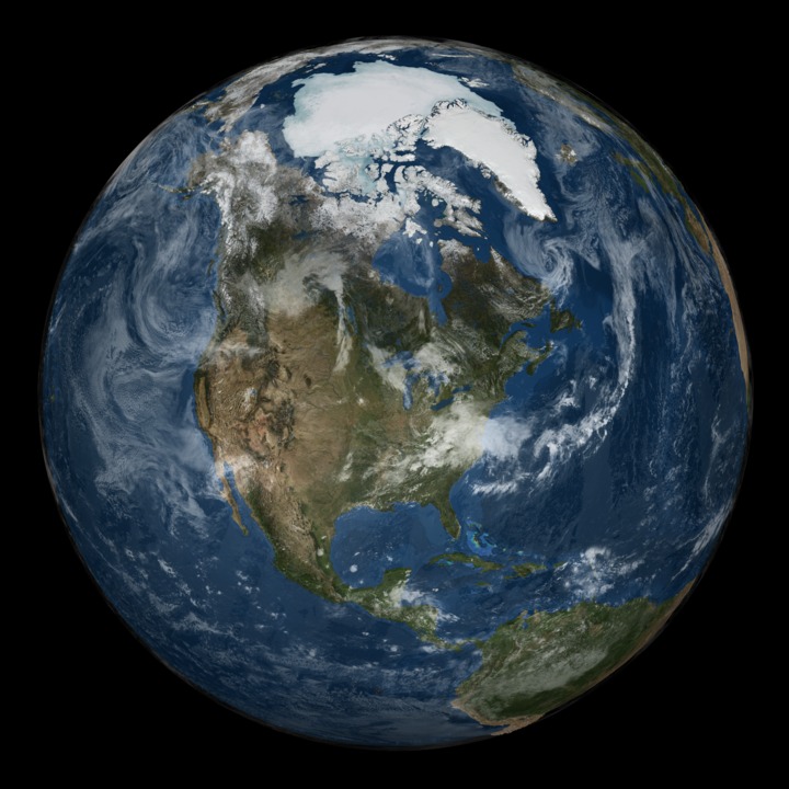
Global View of the Arctic and Antarctic on September 21, 2005
Go to this pageIn support of International Polar Year, this matching pair of images showing a global view of the Arctic and Antarctic were generated in poster-size resolution. Both images show the sea ice on September 21, 2005, the date at which the sea ice was at its minimum extent in the northern hemisphere. The color of the sea ice is derived from the AMSR-E 89 GHz brightness temperature while the extent of the sea ice was determined by the AMSR-E sea ice concentration. Over the continents, the terrain shows the average land cover for September, 2004. (See Blue Marble Next Generation) The global cloud cover shown was obtained from the original Blue Marble cloud data distributed in 2002. (See Blue Marble:Clouds) A matching star background is provided for each view. All images include transparency, allowing them to be composited on a background. ||
- ID: 3673 Visualization
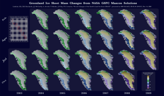
Poster of Greenland Ice Sheet Mass Changes from NASA GSFC GRACE Mascon Solutions
Go to this pageLuthcke, S.B., D.D. Rowlands, J.J. McCarthy, A. Arendt, T. Sabaka, J.P. Boy, F.G. Lemoine, "Recent Changes of the Earth's Land Ice from GRACE, " presented at 2009 Fall AGU, H13G-02 (693337), Dec. 14, 2009.The mass changes of the Greenland Ice Sheet (GIS) are computed from the Gravity Recovery and Climate Experiment (GRACE) inter-satellite range-rate observations for the period April 5, 2003 - July 25, 2009. The mass of the GIS has been computed at 10-day intervals and 200 km spatial resolution from a regional high-resolution mascon solution (Luthcke and others, 2008 and 2006). The poster shows the change in mass during February, April, July and October from 2003 through 2009 as referenced from April 5, 2003. The spatial variation in surface mass is shown in centimeters equivalent height of water. The chart shown in the upper left corner presents total ice loss in Greenland over the same time period measured in gigatons. Corresponding author:Scott B. LuthckeNASA GSFCPlanetary Geodynamics Laboratory, Code 698Scott.B.Luthcke@nasa.gov ||
- ID: 3525 Visualization
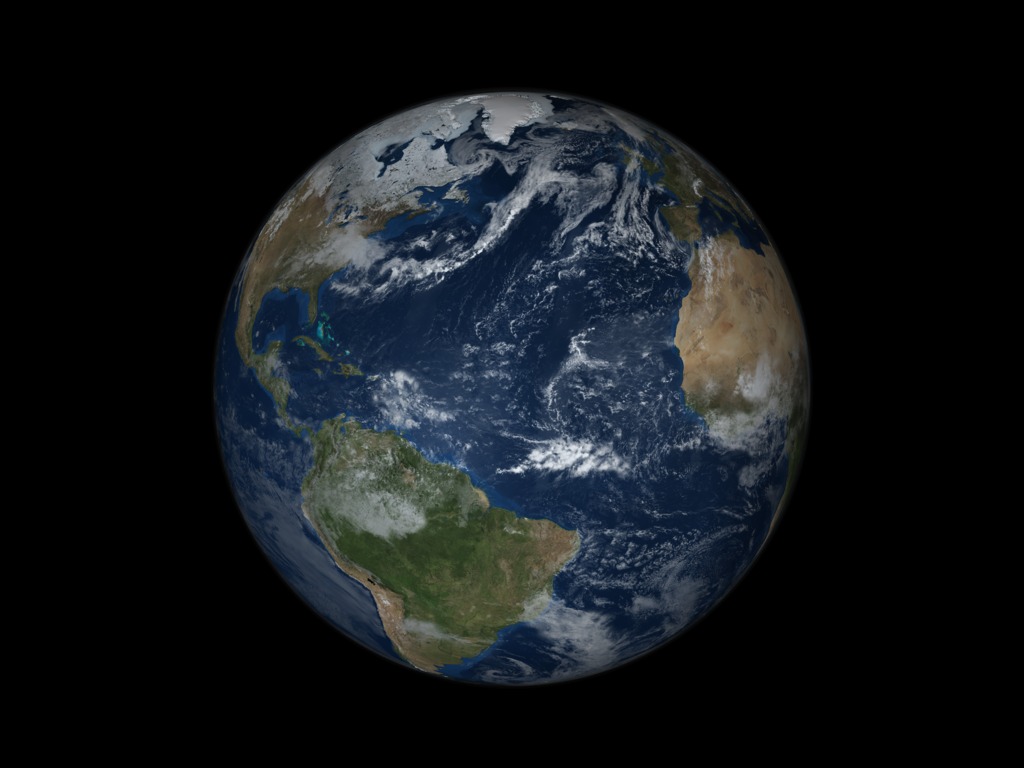
Two Posters of Earth with Sea Ice and Clouds over a Star Background
Go to this pageThese very high resolution images show a global view of the Earth at different orientations with Arctic sea ice on December 8,2008 and September 15, 2008. The extent of the sea ice was determined by the AMSR-E sea ice concentration data. The terrain shows the average land cover for the related months over the continents. (See Blue Marble Next Generation) The global cloud cover shown was obtained from the original Blue Marble cloud data distributed in 2002. (See Blue Marble:Clouds) A matching star background is provided. ||