Cryospheric Videos
Satellites and Instrumentation
- ID: 2978 Visualization
ICESat Lithograph
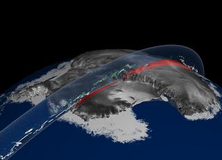
Go to this pageThis still image was generated to be printed as a lithograph for public distribution. [from the litho:] This image illustrates ice sheet elevation and cloud data from ICESat's Geoscience Laser Altimeter System (GLAS) on its first day of operation, February 20, 2003. On that day, the instrument collected a 1064 nm wavelength profile across Antarctica: the lower West Antarctic Ice Sheet in the foreground is separated from the higher East Antarctic Ice Sheet in the background by the steep TransAntarctic Mountains. The elevation profile (in red) is depicted relative to the Earthandapos;s standard ellipsoid with 50x vertical exaggeration. Data collected across floating sea ice and open water of the adjacent Southern Ocean cannot be shown at this scale. Clouds of various thicknesses are indicated by colors changing progressively from light blue (thin clouds) to white (opaque layers). Note that the laser cannot penetrate the thickest clouds causing gaps in the elevation profile below. The RADARSAT (Canadian Space Agency) mosaic is used to illustrate the Antarctic continent. ||
Arctic Sea Ice
- ID: 4138 Visualization
Cover Candidate for PNAS:Albedo Decrease Linked to Arctic Sea Ice
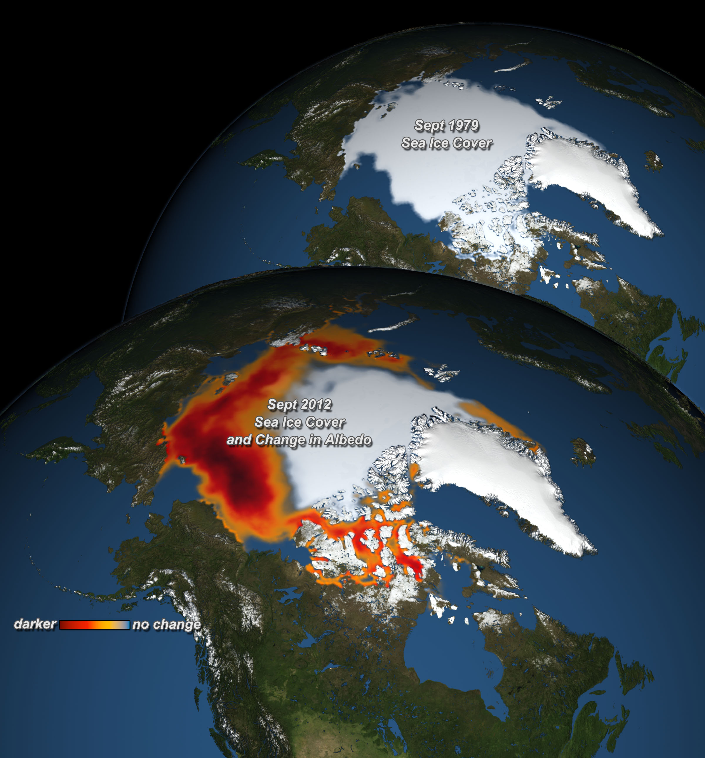
Go to this pageThese still images were generated to be cover candidates for the Proceedings of the National Academy of Sciences (PNAS). The images display data from the paper "Observational determination of albedo decrease caused by vanishing Arctic sea ice". Average September Arctic sea ice from 1979 is shown on the top globe of each image. Average September Arctic sea ice from 2012 with change in albedo overlaid is shown in the bottom globe of each image. Two images are provided which use different color tables.This is the first study to document Arctic-wide decrease in planetary albedo using satellite radiation budget measurements and sea ice data. The study finds a very strong correlation between sea ice cover and planetary albedo.Here are links to the related NASA press release and the article. ||
- ID: 30005 Hyperwall Visual
AMSR-E Sea Ice
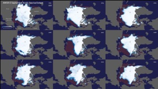
Go to this pageMontage of September sea ice minimum in the Arctic Ocean from 2003 to 2011. || amsre_sept_seaice_2003-2011_print.jpg (1024x575) [145.3 KB] || amsre_sept_seaice_2003-2011.png (4104x2304) [2.3 MB] || amsre_sept_seaice_2003-2011_web.jpg (319x179) [50.4 KB] || amsre_sept_seaice_2003-2011_thm.png (80x40) [6.2 KB] || amsre_sept_seaice_2003-2011_web_searchweb.jpg (320x180) [22.8 KB] ||
Antarctic Ice Sheet
- ID: 3395 Visualization
Jakobshavn Glacier Calving Front Recession from 1850 to 2006
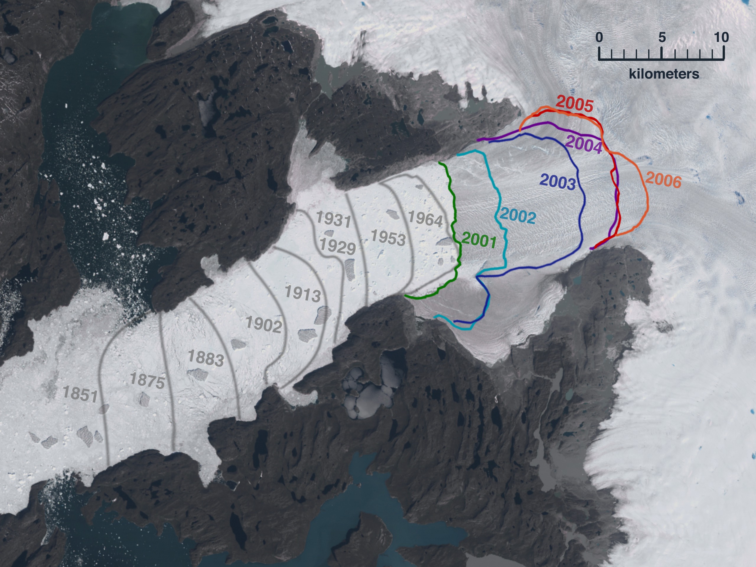
Go to this pageJakobshavn Isbrae is located on the west coast of Greenland at Latitude 69 N. The ice front, where the glacier calves into the sea, receded more than 40 km between 1850 and 2006. Between 1850 and 1964 the ice front retreated at a steady rate of about 0.3 km/yr, after which it occupied approximately the same location until 2001, when the ice front began to recede again, but far more rapidly at about 3 km/yr. After 2004, the glacier began retreating up its two main tributaries: one to the north, and a more rapid one to the southeast. These changes are important for many reasons. As more ice moves from glaciers on land into the ocean, it causes a rise in sea level. Jakobshavn Isbrae is Greenland's largest outlet glacier, draining 6.5 percent of Greenland's ice sheet area. The ice stream's speed-up and near-doubling of the ice flow from land into the ocean has increased the rate of sea level rise by about .06 millimeters (about .002 inches) per year, or roughly 4 percent of the 20th century rate of sea level increase. ||
Snow
- ID: 3934 Visualization
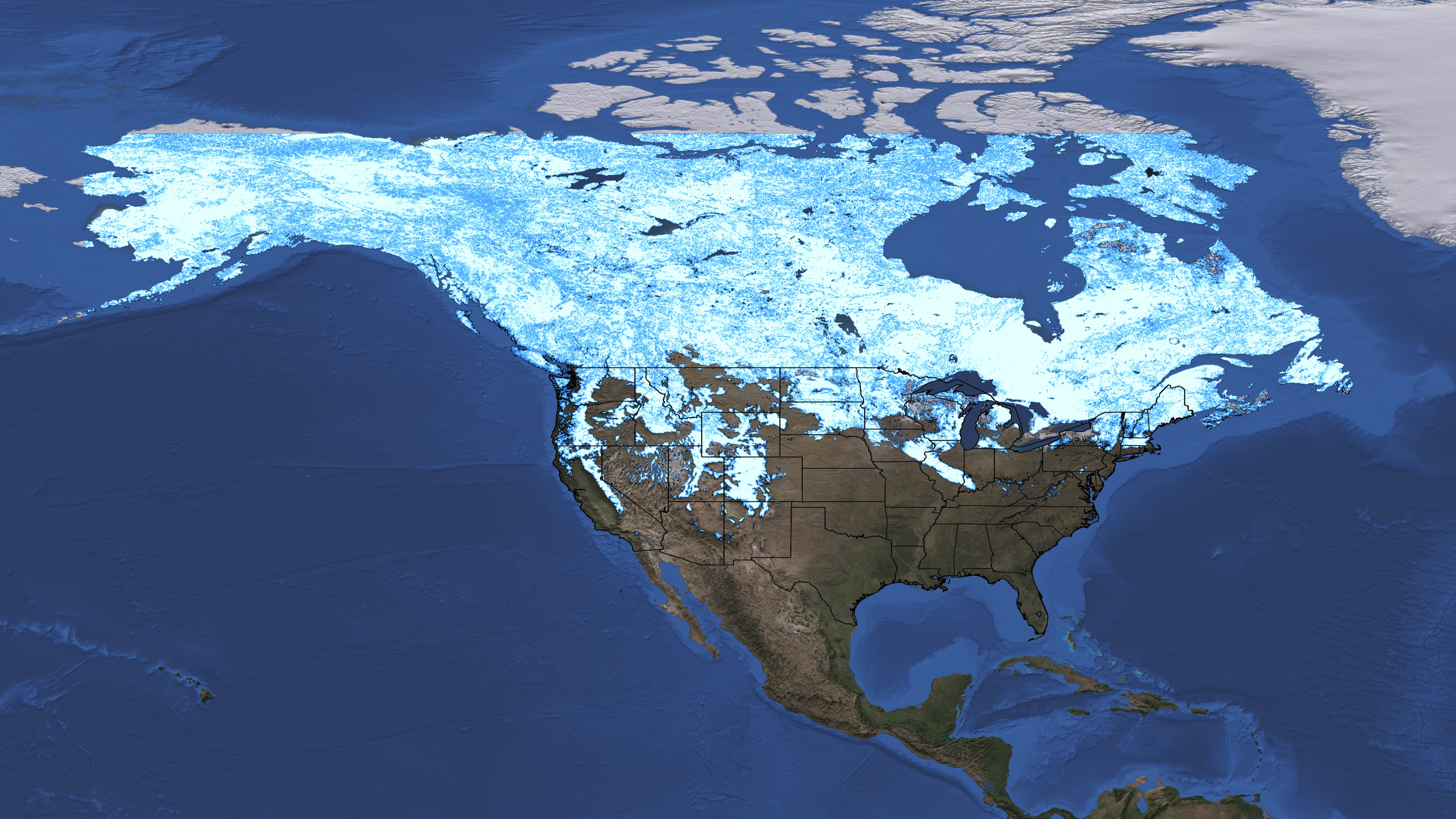
North America Snow Cover Maps
Go to this pageThis entry contains Snow Cover Maps for Norh America with statelines, using the MODIS Cloud-gap-filled (CGF) Product at ~25-km resolution. The MODIS CGF product seeks to provide clear snow observations by filling cloudy areas on a given day with clear observations from previous days.The usual source for this product is the MOD10C1 MODIS/Terra Snow Cover Daily L3 Global 0.05Deg CMG, Version 5 and a variant has been coded that can use MOD10A1 MODIS/Aqua Snow Cover Daily L3 Global 500m Grid, Version 5 as source. Maps are provided for various dates for 2006, 2010, 2011 and 2012, to compare snow cover between years. ||
Greenland Ice Sheet
- ID: 3806 Visualization

Orthographic View of Jakobshavn Calving Front: 1851 to 2010
Go to this pageThe Jakobshavn Isbrae glacier, also known as Sermeq Kujalleq, is located on the west coast of Greenland at Latitude 69 degrees N. The ice front, where the glacier calves into the sea, receded more than 40 km between 1850 and 2010. Between 1850 and 1964 the ice front retreated at a steady rate of about 0.3 km/yr, after which it occupied approximately the same location until 2001, receding 10km in three years. After 2005 the single icefront had retreated enough to split into distinct fronts for the smaller, northern tributary and the main southern trunk. The icestream flows in a deep trough which ends near the current glacier terminus. The bedrock topography is expected to stabilize the location of the icefront for the near future as the glacier continues to drawn ice from Greenland's interior. The movement of ice from glaciers on land into the ocean contributes to a rise in sea level. Jakobshavn Isbrae is Greenland's largest outlet glacier, draining 6.5 percent of Greenland's ice sheet area. This image is generated with an orthographic camera set to view the range from 51.372 W longitude to 49.212 W and from 68.94 N latitude to 69.39 N. The Landsat image shown in the background is a false color image of data collected on July 29, 2009. ||
- ID: 3455 Visualization
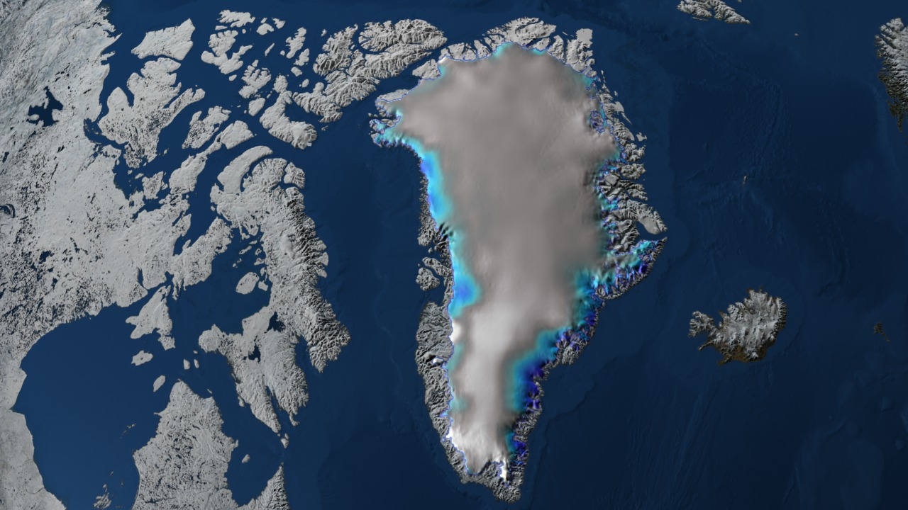
Nadir View of Change in Elevation over Greenland with a Blue/Yellow Color Scale
Go to this pageChanges in the Greenland and Antarctic ice sheets are critical in quantifying forecasts for sea level rise. Since its launch in January 2003, the ICESat elevation satellite has been measuring the change in thickness of these ice sheets. This image of Greenland shows the changes in elevation over the Greenland ice sheet between 2003 and 2006. Gray areas indicate no change in elevation. The white regions indicate a slight thickening, while the blue and purple shades indicate a thinning of the ice sheet. ||
- ID: 3395 Visualization
Jakobshavn Glacier Calving Front Recession from 1850 to 2006
Go to this pageJakobshavn Isbrae is located on the west coast of Greenland at Latitude 69 N. The ice front, where the glacier calves into the sea, receded more than 40 km between 1850 and 2006. Between 1850 and 1964 the ice front retreated at a steady rate of about 0.3 km/yr, after which it occupied approximately the same location until 2001, when the ice front began to recede again, but far more rapidly at about 3 km/yr. After 2004, the glacier began retreating up its two main tributaries: one to the north, and a more rapid one to the southeast. These changes are important for many reasons. As more ice moves from glaciers on land into the ocean, it causes a rise in sea level. Jakobshavn Isbrae is Greenland's largest outlet glacier, draining 6.5 percent of Greenland's ice sheet area. The ice stream's speed-up and near-doubling of the ice flow from land into the ocean has increased the rate of sea level rise by about .06 millimeters (about .002 inches) per year, or roughly 4 percent of the 20th century rate of sea level increase. ||
Other Glaciers
- ID: 4053 Visualization
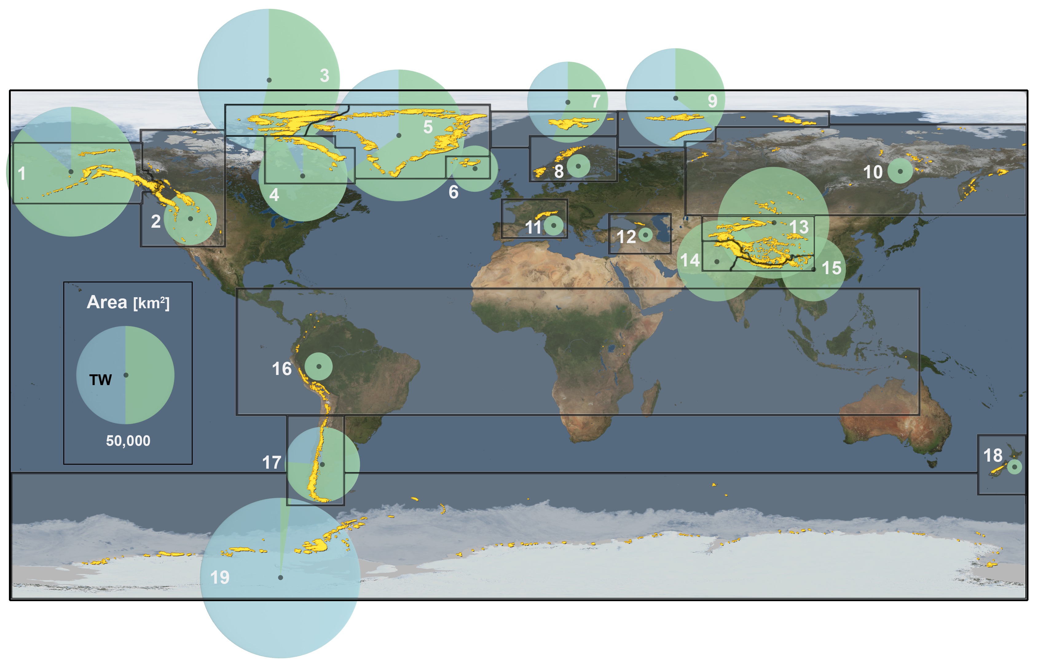
Regional Assessments of Glacier Mass
Go to this pageIn this image, which serves as Figure 4-8 in the Fifth Assessment Report of the Intergovernmental Panel on Climate Change (IPCC), the size of the green circles depicts total area covered by glaciers in each region with the tidewater basin fractions [TW] shown separately in blue. The Randolph Glacier Inventory (RGI) regions, designated by the white number, are referenced in Table 4.2 in the IPCC report. The geographic locations of all glaciers, evident primarily in mountainous regions and high latitudes, are shown in yellow with their area increased to improve visibility. Glacier locations and areas were obtained from airborne and Landsat ETM+, ASTER or SPOT5 satellite imagery and are from the Randolph Glacier Inventory Version 2.0 (Arendt et al., 2012).For additional information, refer to the paper available here. ||
Other
- ID: 30293 Hyperwall Visual
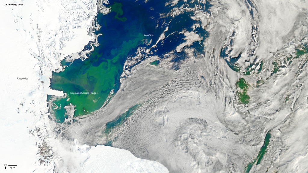
Bloom in the Ross Sea
Go to this pageEvery southern spring and summer the Ross Sea bursts with life. Floating, microscopic plants, known as phytoplankton, soak up the sunlight and the nutrients and grow into prodigious blooms. Those blooms become a great banquet for krill, fish, penguins, whales, and other marine species. This true-color image captures such a bloom in the Ross Sea on January 22, 2011. Bright greens of plant-life have replaced the deep blues of open ocean water. The Ross Sea is a relatively shallow bay in the Antarctic coastline and due south from New Zealand. As the spring weather thaws the sea ice around Antarctica, areas of open water surrounded by ice—polynyas—open up on the continental shelf. In this open water, sunlight provides the fuel and various current systems provide nutrients from deeper waters to form blooms that can stretch 100 to 200 kilometers (60 to 120 miles). These blooms are among the largest in extent and abundance in the world. ||