Heliophysics Education Resources
Overview
Visualizations useful for illustrating key concepts.
Heliospheric Physics
- ID: 20192 Animation
Space Weather
Go to this pageThis movie takes us on a space weather journey from the center of the sun to solar eruptions in the sun's atmosphere all the way to the effects of that activity near Earth. The view starts in the core of the sun where atoms fuse together to create light and energy. Next we travel toward the sun's surface, watching loops of magnetic fields rise up to break through the sun's atmosphere, the corona. In the corona is where we witness giant bursts of radiation and energy known as solar flares, as well as gigantic eruptions of solar material called coronal mass ejections or CMEs. The movie follows one of these CME's toward Earth where it impacts and compresses Earth's own protective magnetic bubble, the magnetosphere. As energy and particles from the sun funnel along magnetic field lines near Earth, they ultimately produce aurora at Earth's poles. ||
- ID: 3551 Visualization

The Coronal Mass Ejection strikes the Earth!
Go to this pageThis visualization is the sequel to animation ID 3867.The CME we saw before continues to expand from the Sun, and its outer boundary is approaching the Earth. Will the Earth be pummeled like its sister planet, Venus?Not this time, for the Earth has a fairly strong geomagnetic field.The geomagnetic field helps deflect the incoming blast of solar particles around the Earth, dramatically reducing the impact of the event.It is important to note that the flowing material of the CME are actually ions and electrons far too small to see. This visualization tries to represent the motions of these tiny particle in a form large enough for us to see.Technical DetailsThis is the dome show component where the CME strikes the Earth.The domemaster format was created by rendering 7 separate camera tiles. The tiles were then stitched together to form final domemaster layers at 4096x4096 resolution and 16 bits per channel with premultiplied alpha and no gamma correction. There are 2 domemaster layers that should be composited as follows:- Earth, Sun and particles- star field (no alpha channel)In addition to the final domemaster frames and movies, the individual camera tiles are included as well. Each domemaster layer has a set of camera tiles. There are 7 cameras numbered 00 through 06 that represent the itiles. Camera 00 is in the center of the domemaster, camera 01 is looking below camera 00, cameras 01 through 06 look around the outside of the dome master in counter-clockwise order. These frames are probably only useful if a better re-stitching algorithm is ever required to be run on the tiles. ||
- ID: 3867 Visualization
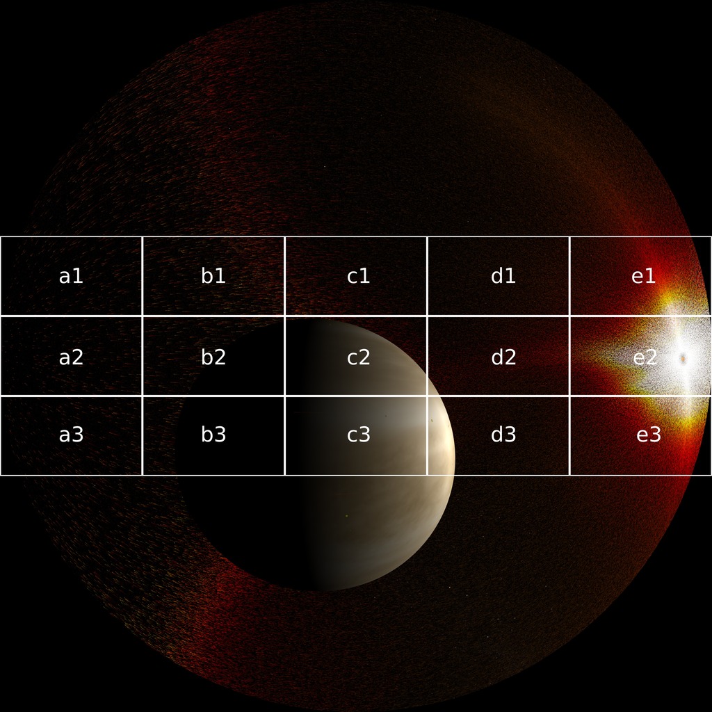
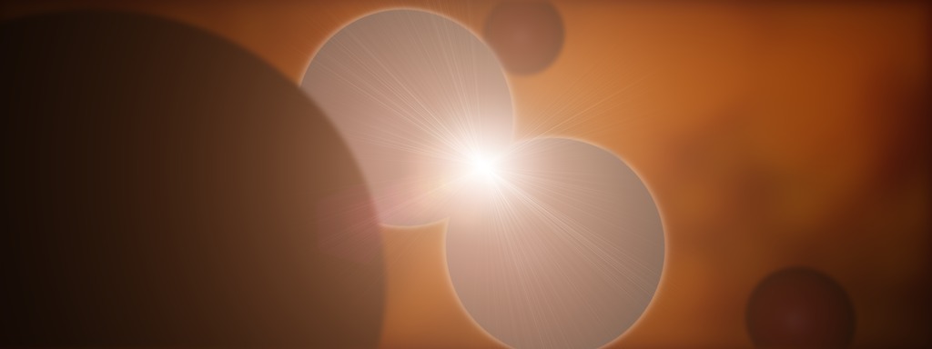
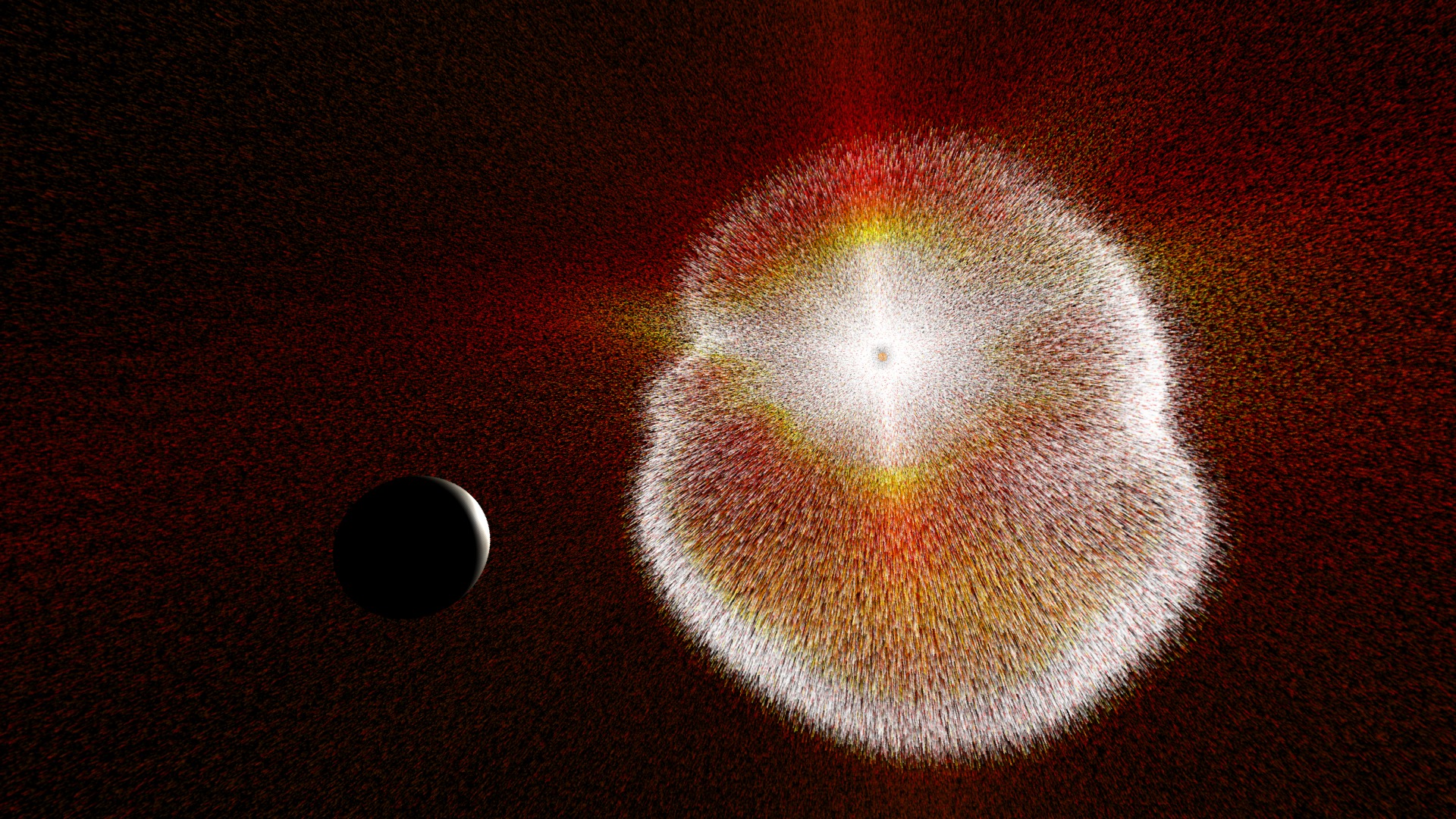
A Coronal Mass Ejection strikes Venus!
Go to this pageEnergetic events on the Sun have impacts throughout the Solar System. This visualization, developed for the "Dynamic Earth" dome show, opens with a closeup view of the Sun. The solar imagery was collected from the Solar Dynamics Observatory (SDO) using an ultraviolet filter (wavelength 304 Ångstroms or 30.4 nanometers). We can observe jets of ionized gases, called prominences, erupting from the solar surface, and often constrained to loop-shaped trajectories due to the solar magnetic field.We pull out from the Sun to reveal the solar wind, which continuously streams outward from the Sun.We eventually reach the orbit of the planet Venus, the solar wind still streaming around us.But a massive eruption, called a coronal mass ejection, or CME, takes place on the Sun, sending a much higher density of particles (ions and electrons) outward into the solar wind.The wave of particles eventually strikes the planet Venus. But Venus has no significant magnetic field, and the particles make it directly to the atmosphere of the planet. These energetic solar events slowly blow away the atmosphere of the planet.The next part of this sequence is "The Coronal Mass Ejection strikes the Earth!".Technical DetailsThis is the dome show component moving from the Sun to Venus being hit by the CME.The domemaster format was created by rendering 7 separate camera tiles. The tiles were then stitched together to form final domemaster layers at 4096x4096 resolution and 16 bits per channel with premultiplied alpha and no gamma correction. There are 3 domemaster layers that should be composited as follows:- Earth and orbits- Sun- star field (no alpha channel)In addition to the final domemaster frames and movies, the individual camera tiles are included as well. Each domemaster layer has a set of camera tiles. There are 7 cameras numbered 00 through 06 that represent the itiles. Camera 00 is in the center of the domemaster, camera 01 is looking below camera 00, cameras 01 through 06 look around the outside of the dome master in counter-clockwise order. These frames are probably only useful if a better re-stitching algorithm is ever required to be run on the tiles. ||
Space Weather
- ID: 3956 Visualization
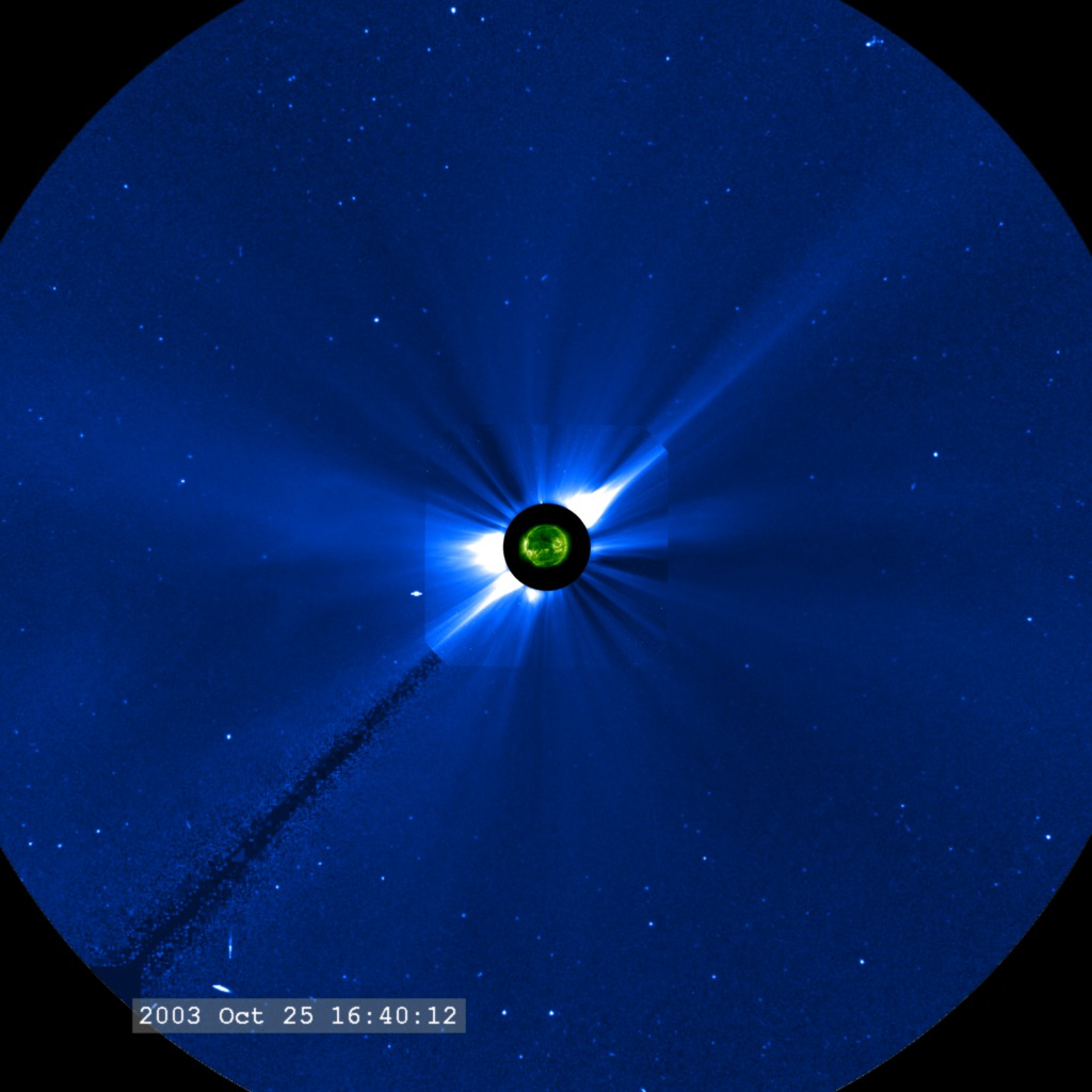
Halloween Solar Storms - 2003
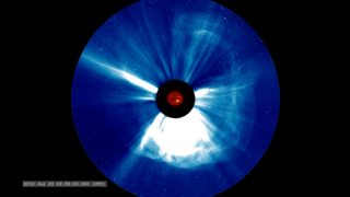
Go to this pageThis is a 1024x1024 pixel version of solar storms providing a more complete view of the SOHO/LASCO/C3 field-of-view.Here is a view of the solar disk in 195 Å ultraviolet light (colored green in this movie) and the Sun's extended atmosphere, or corona, (blue and white in this movie). The corona is visible to the SOHO/LASCO coronagraph instruments, which block the bright disk of the Sun so the significantly fainter corona can be seen. In this movie, the inner coronagraph (designated C2) is combined with the outer coronagraph (C3). This movie covers a two week period in October and November 2003 which exhibited some of the largest solar activity events since the advent of space-based solar observing.As the movie plays, we can observe a number of features of the active Sun. Long streamers radiate outward from the Sun and wave gently due to their interaction with the solar wind. The bright white regions are visible due to their high density of free electrons which scatter the light from the photosphere towards the observer. Protons and other ionized atoms are there as well, but are not as visible since they do not interact with photons as strongly as electrons. Coronal Mass Ejections (CMEs) are occasionally observed launching from the Sun. Some of these launch particle events which can saturate the cameras with snow-like artifacts.Also visible in the coronagraphs are stars and planets. Stars are seen to drift slowly to the right, carried by the relative motion of the Sun and the Earth. The planet Mercury is visible as the bright point moving left of the Sun. The horizontal 'extension' in the image is called 'blooming' and is due to a charge leakage along the readout wires in the CCD imager in the camera. ||
- ID: 3566 Visualization
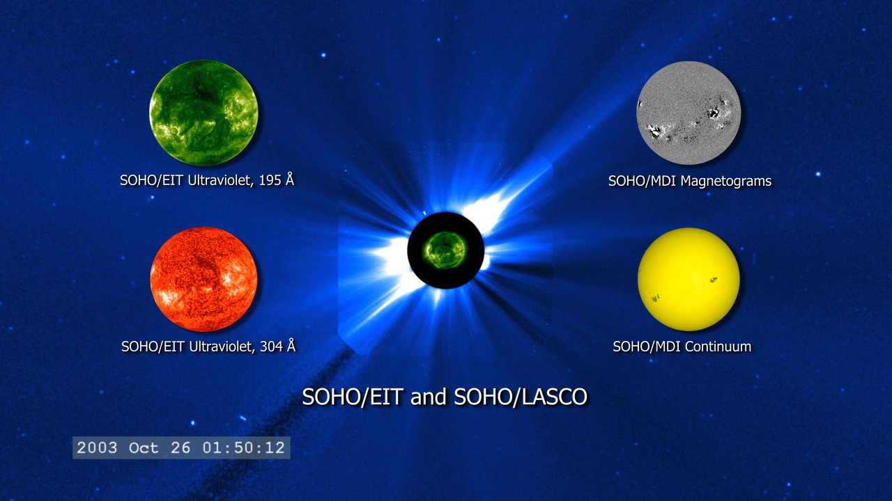
Multi-Sun Composition
Go to this pageThis movie is a composition of multiple solar datasets synchronized in time. The time frame is late October and early November of 2003, the time of some record-breaking solar activity.The background of the movie shows the view of the wide-angle coronagraphs (blue/white), or LASCO instruments, aboard SOHO. They show streams of electrons outbound from the Sun, part of the solar atmosphere. The central green image is the Sun in ultraviolet light from the EIT instrument. Note that flashes of solar flares in the ultraviolet quickly propagate out from the Sun and are visible in LASCO. These events are coronal mass ejections, or CMEs.Overlaid on the upper left is a better view of the EIT ultraviolet image at a wavelength of 195 angstroms (19.5 nanometers).On the lower left, the orange movie is the EIT ultraviolet movie at 304 angstroms (30.4 nanometers).On the upper right is a solar magnetogram, taken by the MDI instrument. The white regions correspond to positive (north) magnetic flux and the dark regions to negative (south) magnetic flux.The colors for the sequences above are not real. They are chosen by convention since the properties recorded by the cameras are not visible to the human eye.The final image on the lower right is also from MDI. It is a combination of several optical wavelengths and is the best representation from SOHO of the Sun in visible light, as we would see it through ground-based telescopes.The movies that are part of this composition are also available individually on the SVS site: Halloween Solar Storms 2003: SOHO/EIT and SOHO/LASCOHalloween Solar Storms 2003: SOHO/EIT Ultraviolet, 195 angstromsHalloween Solar Storms 2003: SOHO/EIT Ultraviolet, 304 angstromsHalloween Solar Storms 2003: SOHO/MDI ContinuumHalloween Solar Storms 2003: SOHO/MDI Magnetograms ||
- ID: 4469 Visualization
Dynamic Earth-A New Beginning
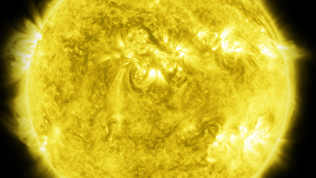
Go to this pageThe visualization 'Excerpt from "Dynamic Earth"' has been one of the most popular visualizations that the Scientific Visualization Studio has ever created. It's often used in presentations and Hyperwall shows to illustrate the connections between the Earth and the Sun, as well as the power of computer simulation in understanding those connections.There is one part of this visualization, however, that has always seemed a little clumsy to us. The opening shot is a pullback from the limb of the sun, where the sun is represented by a movie of 304 Angstrom images from the Solar Dynamics Observatory (SDO). It is difficult to pull back from the limb of a flat sun image and make the sun look spherical, and the problem was made more difficult because the original sun images were in a spherical dome show format. As a result, the pullback from the sun showed some odd reprojection artifacts.The best solution to this issue was to replace the existing pullout with a new one, one which pulled directly out from the center of the solar disk. For the new beginning, we chose a series of SDO images in the 171 Angstrom channel that show a visible coronal mass ejection (CME) in the lower right corner of the solar disk. Although this is not the specific CME that is seen affecting Venus and Earth later in this visualization, its presence links the SDO animation thematically to the later solar storm. The SDO images were also brightened considerably and tinted yellow to match the common perception of the Sun as a bright yellow object (even though it is actually white).Please go to the original version of this visualization to see the complete credits and additional details. ||
Solar Physics
Additional Useful Resources:Classifying Solar Eruptions
 Link
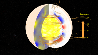
LinkSolar Dynamo
A computer simulation of how the solar magnetic field changes over the course of the 22- year solar cycle.
Go to this link- ID: 4124 Visualization
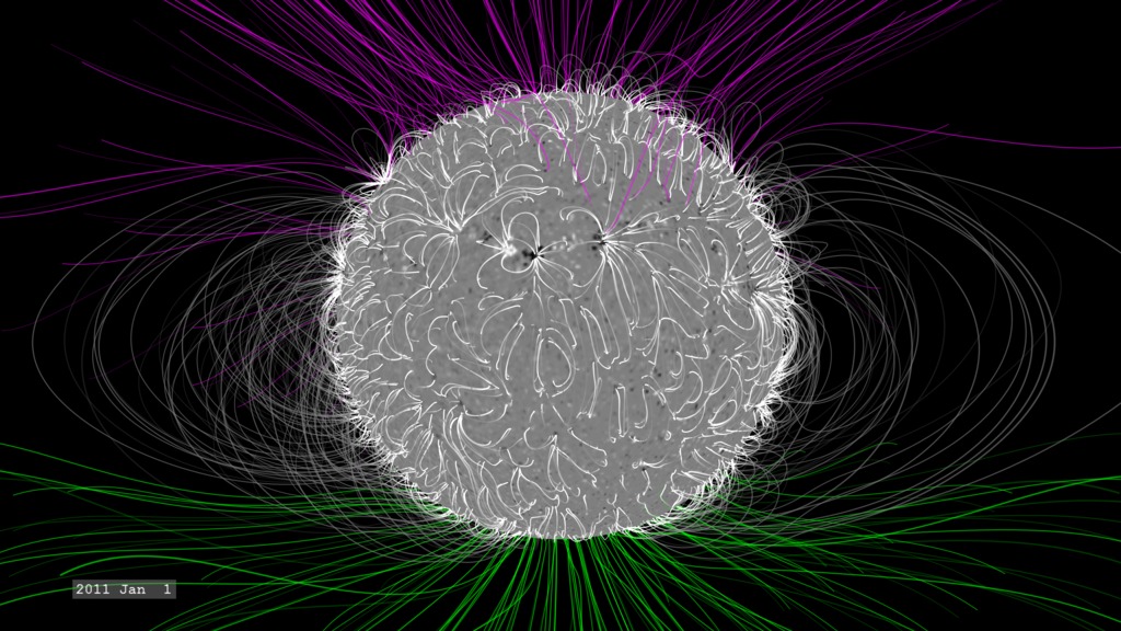
The Sun's Magnetic Field
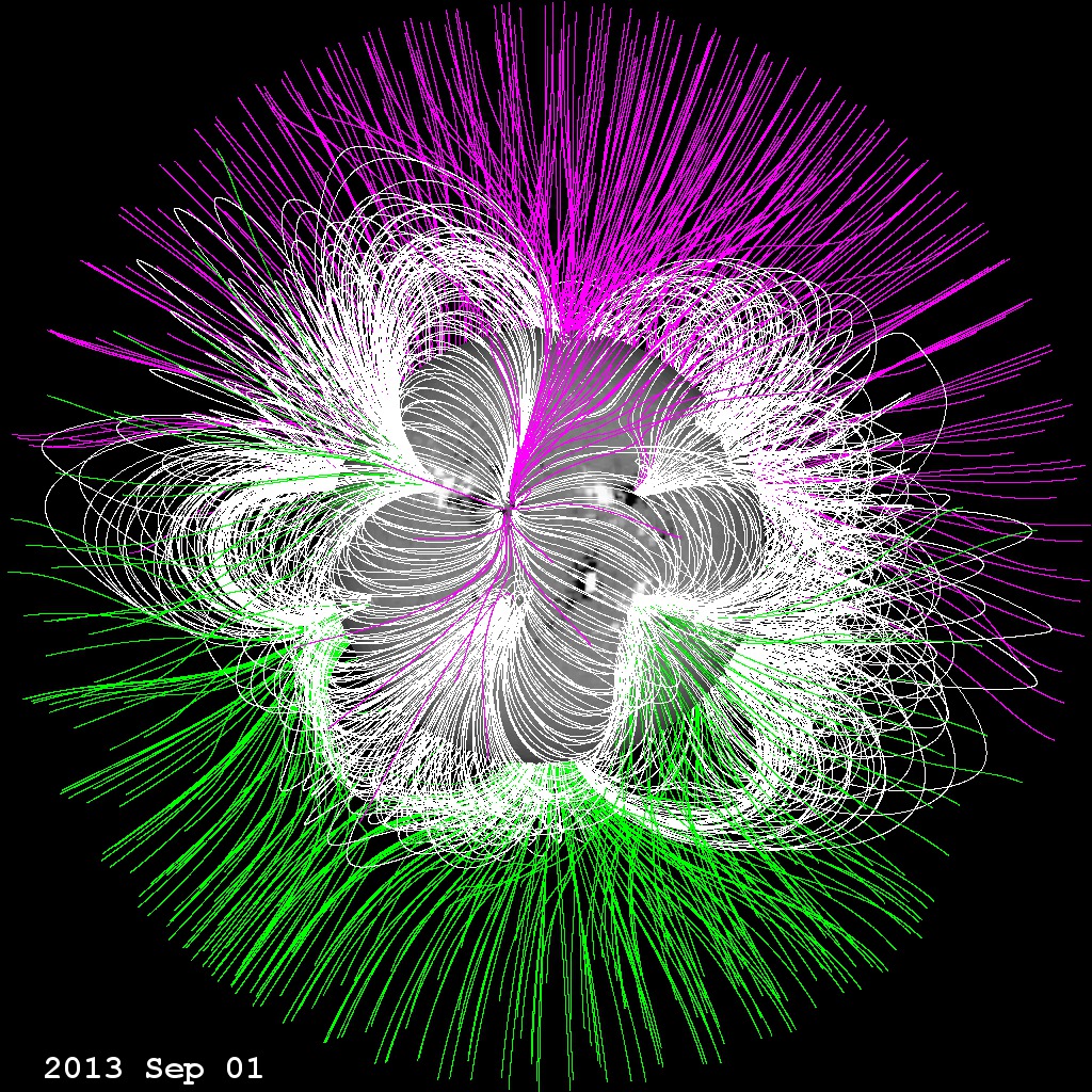
Go to this pageDuring the course of the approximately 11 year sunspot cycle, the magnetic field of the Sun reverses. The last time this happened was around the year 2000. Using magnetograms from the SOHO/MDI and SDO/HMI instruments, it is possible to examine possible configurations of the magnetic field above the photosphere. These magnetic configurations are important in understanding potential conditions of severe space weather.The magnetic field in this animation is constructed using the Potential Field Source Surface (PFSS) model. The PFSS model is one of the simplest yet realistic models we can explore. Using the solar magnetograms as the 'source surface' of the field, it builds the field structure from the photosphere out to about two solar radii (an altitude of 1 solar radius). These visuals were generated using the SolarSoft package. In this visualization, the white magnetic field lines are considered 'closed'. The move up, and then return to the solar surface. The green and violet lines represenent field lines that are considered 'open'. Green represents positive magnetic polarity, and violet represents negative polarity. These field lines do not connect back to the Sun but with more distant magnetic fields in space. These field lines act as easy 'roads' for the high-speed solar wind. ||
 Link
LinkMulti-wavelength Sun
How multiple wavelengths of light provide insight on solar physics
Go to this link Link
LinkSolar Eruptions on Multiple Scales
Solar active events take place on many different spatial and temporal scales.
Go to this link- ID: 4391 Visualization
The Dynamic Solar Magnetic Field
Go to this pageA visualization of the slow changes of the solar magnetic field over the course of four years. || PFSSbasicView_inertial.HD1080i.0400_print.jpg (1024x576) [168.7 KB] || PFSSbasicView_inertial.HD1080i.0400_searchweb.png (180x320) [78.9 KB] || PFSSbasicView_inertial.HD1080i.0400_thm.png (80x40) [5.8 KB] || PFSSbasicView_inertial_1080p30.webm (1920x1080) [18.1 MB] || PFSSbasicView (1920x1080) [128.0 KB] || PFSSbasicView_inertial_1080p30.mp4 (1920x1080) [326.6 MB] || PFSSbasicView_inertial_1080p10.mp4 (1920x1080) [470.2 MB] || PFSSbasicView_HD1080p10.mov (1920x1080) [804.4 MB] || PFSSbasicView_inertial_1080p30.mp4.hwshow [232 bytes] ||
- ID: 4164 Visualization
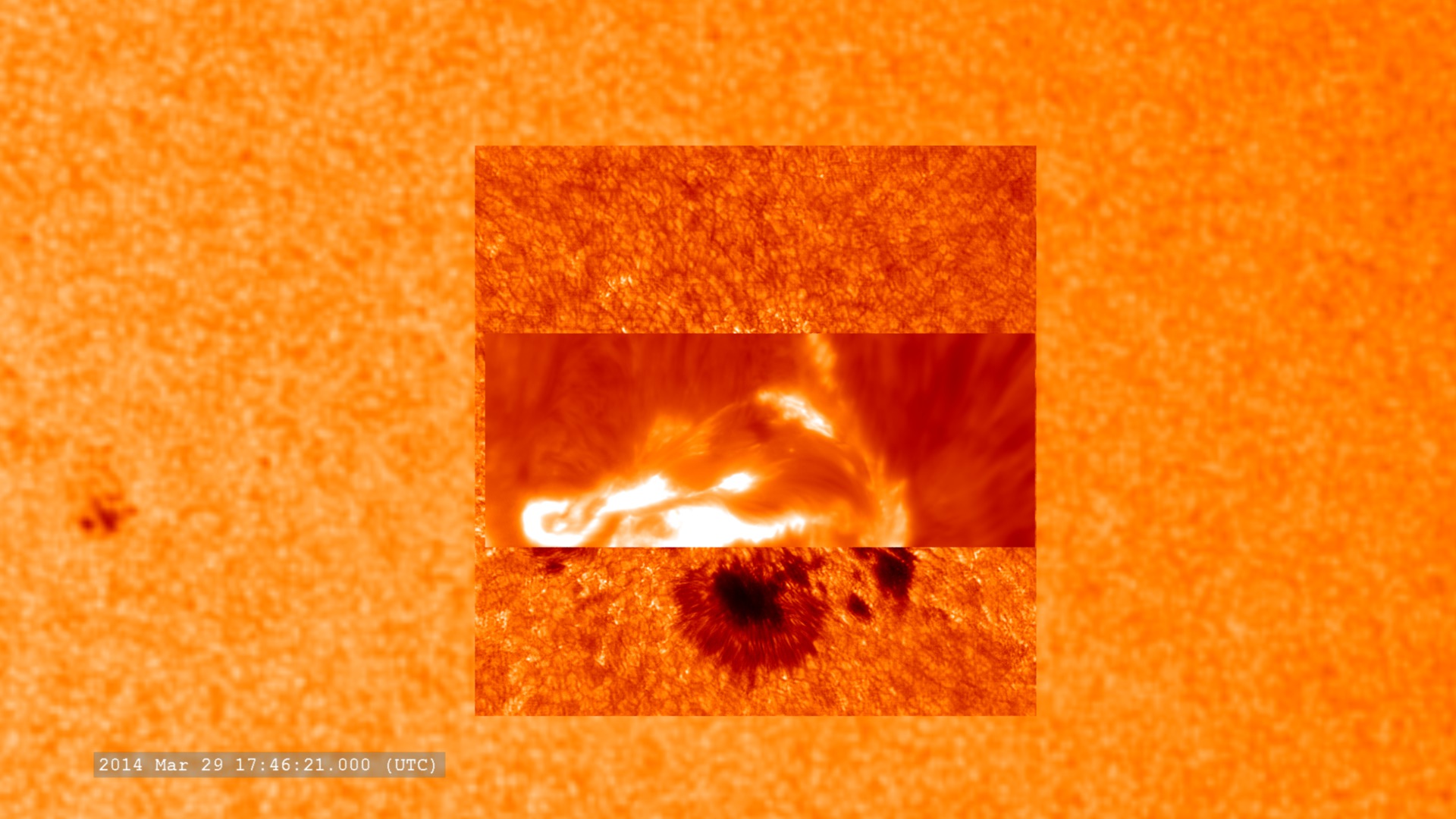
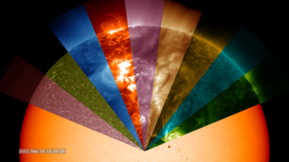
A Multi-Mission View of a Solar Flare: Optical to Gamma-rays
Go to this pageTo improve our understanding of complex phenomena such as solar flares, a wide variety of tools are needed. In the case of astronomy, those tools enable us to analyze the light in many different wavelengths and many different ways.Many different instruments are observing the Sun almost continuously, both from space and on the surface of the Earth. On March 29, 2014, the Dunn Solar Telescope at Sacramento Peak, New Mexico was observing a solar active region and requested other observatories to watch as well. As a result of this coordination, the region was being observed by a large number of different instruments, ground and space-based, when it subsequently erupted with an X-class flare. This visualization presents various combinations of the datasets collected during this effort. The color text represents the dominant color of the dataset in the imagery.Solar Dynamics Observatory (SDO): HMI (617.1nm). This data represents the Sun is visible light similar to how we see it from the ground.Solar Dynamics Observatory (SDO): AIA (17.1nm). Solar ultraviolet emission, which can only be seen from space, reveals plasma flowing, and escaping, along magnetic fields.IRIS Slit-Jaw Imager: 140.0nm. This high-resolution imager also contains a slit (the dark vertical line in the center of the field) which directs the light to an ultraviolet spectrometer which is used to extract even more information about the light. The imager slews back-and-forth across the region, providing spectra over a larger area of the Sun.Hinode/X-ray Telescope: x-ray band. Indicates very hot plasma.RHESSI: 50-100 keV. High-energy gamma-ray emission. Emission from these locations represent the very highest energy photons from the flare event.Dunn Solar Telescope: G-band filter. This filter, showing much of the solar surface (photosphere) in visible light, provides a detailed view of the sunspots and convection cells. The view moves because the instrument was repointed several times during the observation.Dunn Solar Telescope: IBIS ( Hydrogen alpha, 656.3nm; Calcium 854.2 nm; Iron 630.15nm). This is the small rectangular view within the Dunn Solar Telescope G-band view. This instrument can tune the wavelength during the observation, which provides views of the solar atmosphere at different depths. ||
- ID: 4715 Visualization
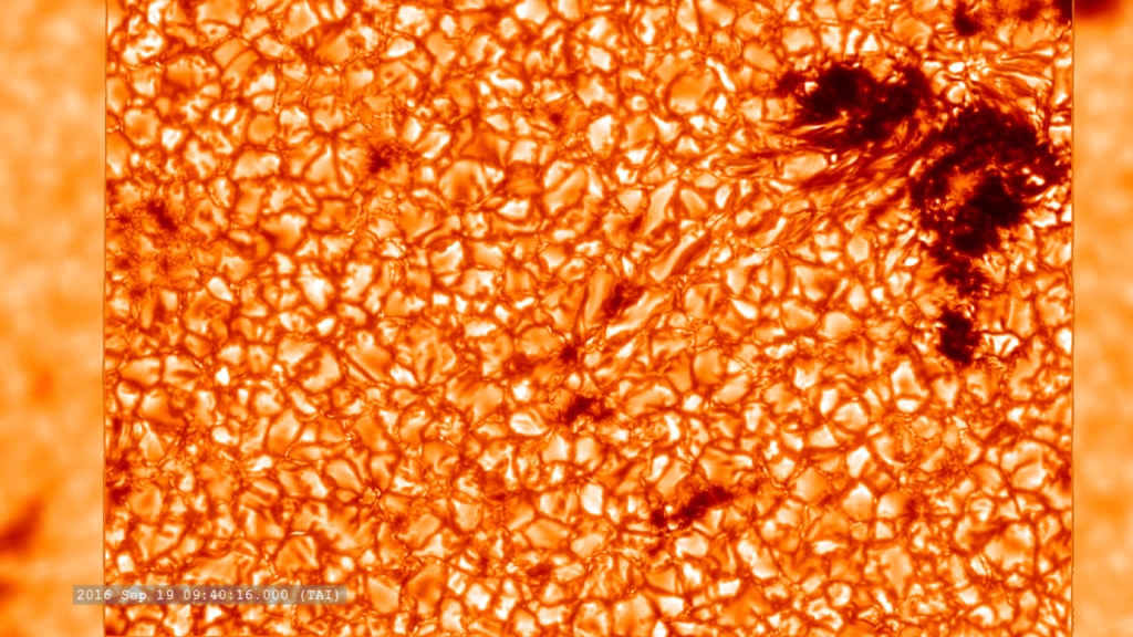
Swedish Solar Telescope: Solar Closeups
Go to this pageClose-up of Active Region 12593 through the 400 nm filter of the Swedish Solar Telescope. SDO/HMI provides the background image. || Sept2016_CHROMIS4000A_stand.HD1080i.00100_print.jpg (1024x576) [200.8 KB] || Sept2016_CHROMIS4000A_stand.HD1080i.00100_searchweb.png (180x320) [136.4 KB] || Sept2016_CHROMIS4000A_stand.HD1080i.00100_thm.png (80x40) [9.1 KB] || SwedishST (1920x1080) [0 Item(s)] || Sept2016_CHROMIS4000A.HD1080i_p30.mp4 (1920x1080) [19.4 MB] || Sept2016_CHROMIS4000A.HD1080i_p30.webm (1920x1080) [1.5 MB] || SwedishST (3840x2160) [0 Item(s)] || Sept2016_CHROMIS4000A.UHD3840_2160p30.mp4 (3840x2160) [50.6 MB] || Sept2016_CHROMIS4000A.HD1080i_p30.mp4.hwshow [199 bytes] ||
Magnetospheric Physics (Earth)
 Link
LinkMagnetospheres vs. CMEs
Space weather modeling helps predict Earth's geomagnetic response to coronal mass ejections.
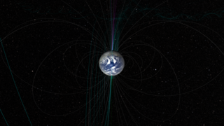
Go to this link- ID: 4141 Visualization
Earth's Magnetosphere
Go to this pageEarth's magnetic field creates a 'bubble' around Earth that helps protect our planet from some of the more harmful effects of energetic particles streaming out from the sun in the solar wind. Some of the earliest hints of this interaction go back to the 1850s with the work of Richard Carrington, and in the early 1900s with the work of Kristian Birkeland and Carl Stormer. That this field might form a type of 'bubble' around Earth was hypothesized by Sidney Chapman and Vincent Ferraro in the 1930s. The term 'magnetosphere' was applied to magnetic bubble by Thomas Gold in 1959. But it wasn't until the Space Age, when we sent the first probes to other planets, that we found clear evidence of their magnetic fields (though there were hints of a magnetic field for Jupiter in the 1950s, due to observations from radio telescopes). The Voyager program , two spacecraft launched in 1977, and successors to the Pioneer 10 and 11 missions, completed flybys of the giant outer planets. They became the implementation of the 'Grand Tour' of the outer planets originally proposed in the late 1960s. The Voyagers provided some of the first detailed measurments of the strength, extent and diversity of the magnetospheres of the outer planets.In these visualizations, we present simplified models of these planetary magnetospheres, designed to illustrate their scale, and basic features of their structure and impacts of the magnetic axes offset from the planetary rotation axes. For this Earth visualization, note that the north magnetic pole points out of the southern hemisphere.For these visualizations, the magnetic field structure is represented by gold/copper lines. Some additional glyphs are provided to indicate some key directions in the field model.The Yellow arrow points towards the sun. The magnetotail is pointed in the opposite direction.The Cyan arrow represents the magnetic axis, usually tilted relative to the rotation axis. The arrow indicates the NORTH magnetic pole (convention has field lines moving north to south as the north pole of bar magnet (and compass pointer) points to the south magnetic pole).The Blue arrow represents the north rotation axis. It is part of the 3-D axis glyph (red, green, and blue arrows) included to make the planetary rotation more apparent.The semi-transparent grey mesh in the distance represents the boundary of the magnetosphere.Major satellites of the planetary system are also included. When appropriate for the time window of the visualization, the Voyager flyby trajectories are indicated.The models are constructed by combining the fields of a simple magnetic dipole, a current sheet (whose intensity is tuned match the scale of the magnetotail), and occasionally a ring current. This is a variation of the simple Luhmann-Friesen magnetosphere model. They are meant to be representative of the basic characteristics of the planetary magnetic fields. Some features NOT included are longitudes of magnetic poles to a standard planetary coordinate system and offsets of the dipole center from the planetary center. ReferencesT. Gold, Motions in the Magnetosphere of the EarthLuhmann and Friesen, A simple model of the magnetosphereLASP: Polarity of planetary magnetic fieldsWikipedia: The Solar Storm of 1859Wikipedia: Kristian BirkelandWikipedia: Carl StørmerSpecial thanks to Arik Posner (NASA/HQ) and Gina DiBraccio (UMBC/GSFC) for helpful pointers on orientation of planetary rotation and magnetic axes. ||
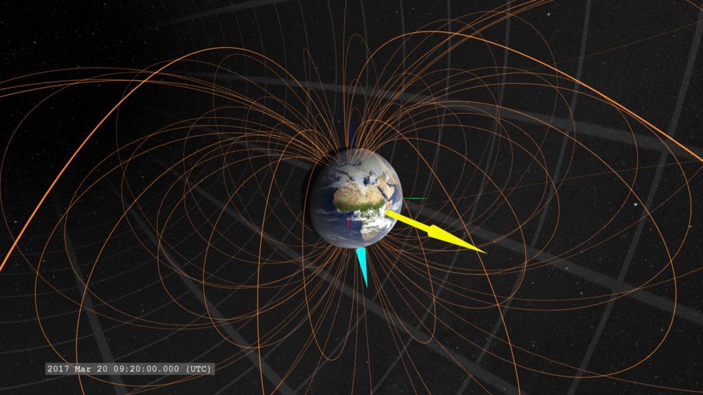
- ID: 3590 Visualization
THEMIS/ASI Nights - High Resolution
Go to this pageA collection of ground-based All-Sky Imagers (ASI) makes an important component of the THEMIS mission in understanding the interaction of the magnetosphere and aurora. It is sometimes referred to as the sixth THEMIS satellite. Descriptions of the instruments are available on the THEMIS-Canada Home Page. Imagery from each camera is co-registered to the surface of the Earth and assembled into a view of the auroral events. This movie presents data from the first large auroral substorm since the THEMIS launch. The substorm reached its maximum between 6:00 and 7:00 UT. Note that the ASI data in this movie are assembled from significantly higher resolution datesets than the earlier version, THEMIS/ASI Nights. The higher resolution enables you to see much finer details in the aurora structure. In addition, one notices trees circling the horizon visible to the cameras located in western Canada. ||
- ID: 20097 Animation
Substorms
Go to this pageThis animation shows a magnetospheric substorm, during which the reconnection causes energy to be rapidly released along the field lines causing the auroras to brighten. ||
- ID: 4217 Visualization
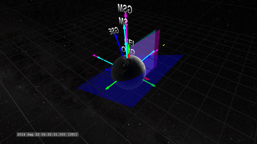
Coordinated Earth: Measuring Space in the Near-Earth Environment
Go to this pageWhen we operate satellites in space, they are often taking measurements along the locations of their travel. As with many measurements, they are only useful if they can be placed in the proper context - their relationship to other measurements at the same, and different, locations. To assemble these measurements within context, we also need to know where and when the measurements were taken, and to do that, we need to define a coordinate system.In three-dimensional space, we define a position with three numbers, relative to a point we define as the Origin of the coordinate system, defined as (0,0,0). Each number represents a distance from the origin along one of three directions. We usually defined these directions by axes, labelled X, Y, and Z, which are defined to be mutually perpendicular, each one is at right angles to the others.While all coordinate systems are equal, all coordinate systems are not equally convenient for a given problem of interest. Sometimes the data and mathematics we use for exploring different problems can be more complex in one coordinate system or another. To simplify this, we often define a number of different coordinate systems and ways to do transformations between them.In studying the space environment around Earth, we find five different coordinate systems of use. Geocentric (GEO): This is the coordinate system useful for measuring things close to Earth’s surface. The origin is chosen at the center of Earth. The x-axis points from the center of Earth through the Prime Meridian (by convention chosen as the meridian in Greenwich, London, UK (longitude = 0). The z-axis points towards the north geographic pole. Geocentric Earth Inertial (GEI): This coordinate system is fixed relative to the distant stars, so Earth rotates about the z-axis relative to it. The origin of this coordinate system is at the center of the Earth. The x-axis points to the first point in Aries (Wikipedia: Vernal Equinox) and the z-axis points to the north geographic & celestial pole. The direction of the celestial pole changes due to Earth’s rotational precession (Wikipedia). Geocentric Solar Ecliptic (GSE): The origin is at the center of the Earth. The x-axis is along the line between Earth and the Sun. The z-axis is the north ecliptic pole and is fixed in direction (but for slow changes due to Earth orbital changes). Solar Magnetic (SM): the origin is at the center of the Earth. The z-axis is chosen parallel to the Earth magnetic dipole axis. The y-axis is chosen to be perpendicular to the z-axis and the Earth-Sun line (pointing towards dusk). Geocentric Solar Magnetospheric (GSM): The origin is at the center of the Earth. The x-axis is defined as the Earth-Sun line (same as in GSE). The y-axis is defined to be perpendicular to the plane containing the x-axis and the magnetic dipole axis so the magnetic axis always lies in this plane.Similar coordinate systems are defined for the Sun and other planets of the Solar System.Development Note: This visualization was originally developed to test coordinate system transformations in the visualization framework.References:C. T. Russell. "Geophysical coordinate transformations". Cosmical Electrodynamics 2, 184-196 (1971). URL.M.A. Hapgood. "Space Physics Coordinate Transformations: A User Guide". Planetary & Space Science, 40, 711-717.(1992). URLSPENVIS Help Pages: Coordinate Systems and transformations ||
- ID: 4241 Visualization
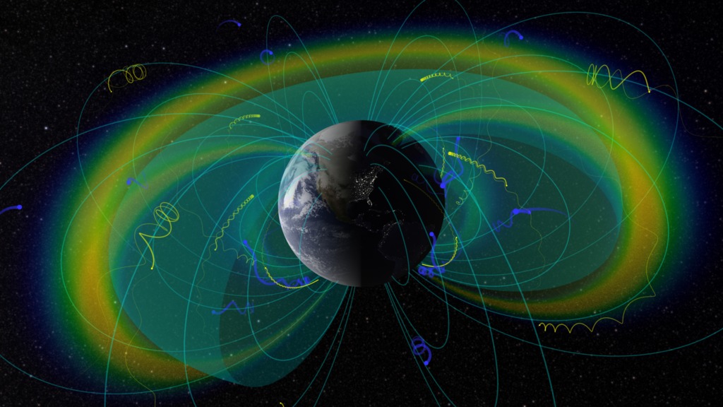
Radiation Belts & Plasmapause
Go to this pageVisualization of the radiation belts with confined charged particles (blue & yellow) and plasmapause boundary (blue-green surface) || Earth_BeltsPlasmapauseParticles_Oblique.noslate_GSEmove.HD1080i.0400_print.jpg (1024x576) [136.6 KB] || Earth_BeltsPlasmapauseParticles_Oblique.noslate_GSEmove.HD1080i.0400_web.png (320x180) [96.2 KB] || Earth_BeltsPlasmapauseParticles_Oblique.noslate_GSEmove.HD1080i.0400_searchweb.png (320x180) [96.2 KB] || Earth_BeltsPlasmapauseParticles_Oblique.noslate_GSEmove.HD1080i.0400_thm.png (80x40) [6.9 KB] || BeltsPlasmapauseParticles_HD1080.mov (1920x1080) [28.3 MB] || Earth_BeltsPlasmapauseParticles_Oblique_HD1080.mp4 (1920x1080) [16.6 MB] || BeltsPlasmapauseParticles_HD720.mov (1280x720) [10.6 MB] || 1920x1080_16x9_30p (1920x1080) [0 Item(s)] || Earth_BeltsPlasmapauseParticles_Oblique_HD1080.webm (960x540) [2.3 MB] || BeltsPlasmapauseParticles_iPod.m4v (640x360) [3.7 MB] || radiation-belts--plasmapause.hwshow [342 bytes] ||
Planetary Magnetospheres
- ID: 4142 Visualization
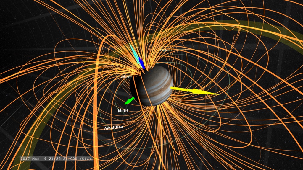
Jupiter's Magnetosphere
Go to this pageEarth's magnetic field creates a 'bubble' around Earth that helps protect our planet from some of the more harmful effects of energetic particles streaming out from the sun in the solar wind. Some of the earliest hints of this interaction go back to the 1850s with the work of Richard Carrington, and in the early 1900s with the work of Kristian Birkeland and Carl Stormer. That this field might form a type of 'bubble' around Earth was hypothesized by Sidney Chapman and Vincent Ferraro in the 1930s. The term 'magnetosphere' was applied to magnetic bubble by Thomas Gold in 1959. But it wasn't until the Space Age, when we sent the first probes to other planets, that we found clear evidence of their magnetic fields (though there were hints of a magnetic field for Jupiter in the 1950s, due to observations from radio telescopes). The Voyager program , two spacecraft launched in 1977, and successors to the Pioneer 10 and 11 missions, completed flybys of the giant outer planets. They became the implementation of the 'Grand Tour' of the outer planets originally proposed in the late 1960s. The Voyagers provided some of the first detailed measurments of the strength, extent and diversity of the magnetospheres of the outer planets.In these visualizations, we present simplified models of these planetary magnetospheres, designed to illustrate their scale, and basic features of their structure and impacts of the magnetic axes offset from the planetary rotation axes. The volcanic activity on Jupiter's moon Io launches a large amount of sulfur-based compounds along its orbit, which is subsequently ionized by solar ultraviolet radiation. This is represented in the visualization by the yellowish structure along the orbit of Io. This creates a plasma torus and ring current around Jupiter, which alters the planet's magnetic field, forming some of the perturbations in Jupiter's magnetic field along the orbit of Io.For these visualizations, the magnetic field structure is represented by gold/copper lines. Some additional glyphs are provided to indicate some key directions in the field model.The Yellow arrow points towards the sun. The magnetotail is pointed in the opposite direction.The Cyan arrow represents the magnetic axis, usually tilted relative to the rotation axis. The arrow indicates the NORTH magnetic pole (convention has field lines moving north to south as the north pole of bar magnet (and compass pointer) points to the south magnetic pole).The Blue arrow represents the north rotation axis. It is part of the 3-D axis glyph (red, green, and blue arrows) included to make the planetary rotation more apparent.The semi-transparent grey mesh in the distance represents the boundary of the magnetosphere.Major satellites of the planetary system are also included. When appropriate for the time window of the visualization, the Voyager flyby trajectories are indicated.The models are constructed by combining the fields of a simple magnetic dipole, a current sheet (whose intensity is tuned match the scale of the magnetotail), and occasionally a ring current. This is a variation of the simple Luhmann-Friesen magnetosphere model. They are meant to be representative of the basic characteristics of the planetary magnetic fields. Some features NOT included are longitudes of magnetic poles to a standard planetary coordinate system and offsets of the dipole center from the planetary center. ReferencesT. Gold, Motions in the Magnetosphere of the EarthLuhmann and Friesen, A simple model of the magnetosphereLASP: Polarity of planetary magnetic fieldsWikipedia: The Solar Storm of 1859Wikipedia: Kristian BirkelandWikipedia: Carl StørmerSpecial thanks to Arik Posner (NASA/HQ) and Gina DiBraccio (UMBC/GSFC) for helpful pointers on orientation of planetary rotation and magnetic axes. ||
- ID: 4143 Visualization
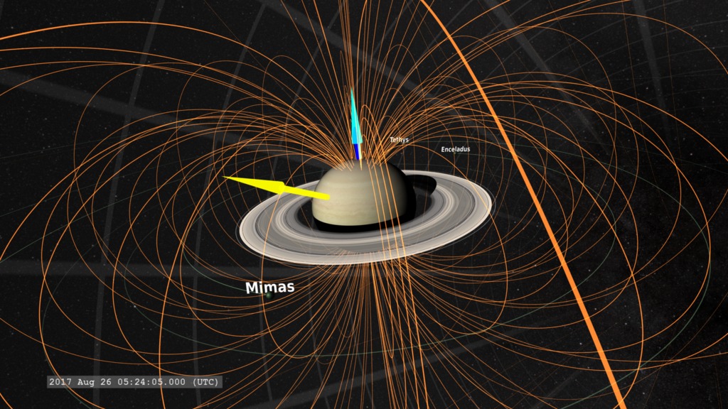
Saturn's Magnetosphere
Go to this pageEarth's magnetic field creates a 'bubble' around Earth that helps protect our planet from some of the more harmful effects of energetic particles streaming out from the sun in the solar wind. Some of the earliest hints of this interaction go back to the 1850s with the work of Richard Carrington, and in the early 1900s with the work of Kristian Birkeland and Carl Stormer. That this field might form a type of 'bubble' around Earth was hypothesized by Sidney Chapman and Vincent Ferraro in the 1930s. The term 'magnetosphere' was applied to magnetic bubble by Thomas Gold in 1959. But it wasn't until the Space Age, when we sent the first probes to other planets, that we found clear evidence of their magnetic fields (though there were hints of a magnetic field for Jupiter in the 1950s, due to observations from radio telescopes). The Voyager program , two spacecraft launched in 1977, and successors to the Pioneer 10 and 11 missions, completed flybys of the giant outer planets. They became the implementation of the 'Grand Tour' of the outer planets originally proposed in the late 1960s. The Voyagers provided some of the first detailed measurments of the strength, extent and diversity of the magnetospheres of the outer planets.In these visualizations, we present simplified models of these planetary magnetospheres, designed to illustrate their scale, and basic features of their structure and impacts of the magnetic axes offset from the planetary rotation axes. For these visualizations, the magnetic field structure is represented by gold/copper lines. Some additional glyphs are provided to indicate some key directions in the field model.The Yellow arrow points towards the sun. The magnetotail is pointed in the opposite direction.The Cyan arrow represents the magnetic axis, usually tilted relative to the rotation axis. The arrow indicates the NORTH magnetic pole (convention has field lines moving north to south as the north pole of bar magnet (and compass pointer) points to the south magnetic pole).The Blue arrow represents the north rotation axis. It is part of the 3-D axis glyph (red, green, and blue arrows) included to make the planetary rotation more apparent.The semi-transparent grey mesh in the distance represents the boundary of the magnetosphere.Major satellites of the planetary system are also included. When appropriate for the time window of the visualization, the Voyager flyby trajectories are indicated.The models are constructed by combining the fields of a simple magnetic dipole, a current sheet (whose intensity is tuned match the scale of the magnetotail), and occasionally a ring current. This is a variation of the simple Luhmann-Friesen magnetosphere model. They are meant to be representative of the basic characteristics of the planetary magnetic fields. Some features NOT included are longitudes of magnetic poles to a standard planetary coordinate system and offsets of the dipole center from the planetary center. ReferencesT. Gold, Motions in the Magnetosphere of the EarthLuhmann & Friesen, A simple model of the magnetosphereLASP: Polarity of planetary magnetic fieldsWikipedia: The Solar Storm of 1859Wikipedia: Kristian BirkelandWikipedia: Carl StørmerSpecial thanks to Arik Posner (NASA/HQ) and Gina DiBraccio (UMBC/GSFC) for helpful pointers on orientation of planetary rotation and magnetic axes. ||
- ID: 4144 Visualization
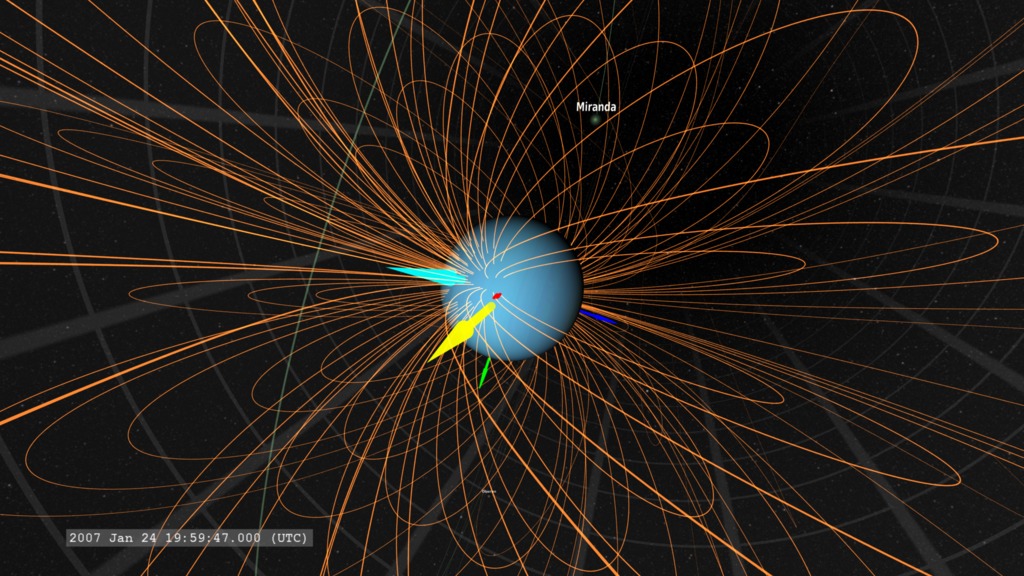
Uranus' Magnetosphere
Go to this pageEarth's magnetic field creates a 'bubble' around Earth that helps protect our planet from some of the more harmful effects of energetic particles streaming out from the sun in the solar wind. Some of the earliest hints of this interaction go back to the 1850s with the work of Richard Carrington, and in the early 1900s with the work of Kristian Birkeland and Carl Stormer. That this field might form a type of 'bubble' around Earth was hypothesized by Sidney Chapman and Vincent Ferraro in the 1930s. The term 'magnetosphere' was applied to magnetic bubble by Thomas Gold in 1959. But it wasn't until the Space Age, when we sent the first probes to other planets, that we found clear evidence of their magnetic fields (though there were hints of a magnetic field for Jupiter in the 1950s, due to observations from radio telescopes). The Voyager program , two spacecraft launched in 1977, and successors to the Pioneer 10 and 11 missions, completed flybys of the giant outer planets. They became the implementation of the 'Grand Tour' of the outer planets originally proposed in the late 1960s. The Voyagers provided some of the first detailed measurments of the strength, extent and diversity of the magnetospheres of the outer planets.In these visualizations, we present simplified models of these planetary magnetospheres, designed to illustrate their scale, and basic features of their structure and impacts of the magnetic axes offset from the planetary rotation axes. The rotation axis of Uranus is tilted over ninety degrees relative to the revolution axis of the solar system, placing it roughly in the plane of the solar system. In addition, the magnetic axis has a large tilt relative to the rotation axis. These effects combine to not only give Uranus a more a more variable magnetosphere, but suggest the planet's magnetic field may be generated by a different mechanism than that of Earth, Jupiter and Saturn.For these visualizations, the magnetic field structure is represented by gold/copper lines. Some additional glyphs are provided to indicate some key directions in the field model.The Yellow arrow points towards the sun. The magnetotail is pointed in the opposite direction.The Cyan arrow represents the magnetic axis, usually tilted relative to the rotation axis. The arrow indicates the NORTH magnetic pole (convention has field lines moving north to south as the north pole of bar magnet (and compass pointer) points to the south magnetic pole).The Blue arrow represents the north rotation axis. It is part of the 3-D axis glyph (red, green, and blue arrows) included to make the planetary rotation more apparent.The semi-transparent grey mesh in the distance represents the boundary of the magnetosphere.Major satellites of the planetary system are also included. When appropriate for the time window of the visualization, the Voyager flyby trajectories are indicated.The models are constructed by combining the fields of a simple magnetic dipole, a current sheet (whose intensity is tuned match the scale of the magnetotail), and occasionally a ring current. This is a variation of the simple Luhmann-Friesen magnetosphere model. They are meant to be representative of the basic characteristics of the planetary magnetic fields. Some features NOT included are longitudes of magnetic poles to a standard planetary coordinate system and offsets of the dipole center from the planetary center. ReferencesT. Gold, Motions in the Magnetosphere of the EarthLuhmann & Friesen, A simple model of the magnetosphereMagnetic reconnection at Uranus' magnetopauseLASP: Polarity of planetary magnetic fieldsWikipedia: The Solar Storm of 1859Wikipedia: Kristian BirkelandWikipedia: Carl StørmerSpecial thanks to Arik Posner (NASA/HQ) and Gina DiBraccio (UMBC/GSFC) for helpful pointers on orientation of planetary rotation and magnetic axes. ||
- ID: 4145 Visualization
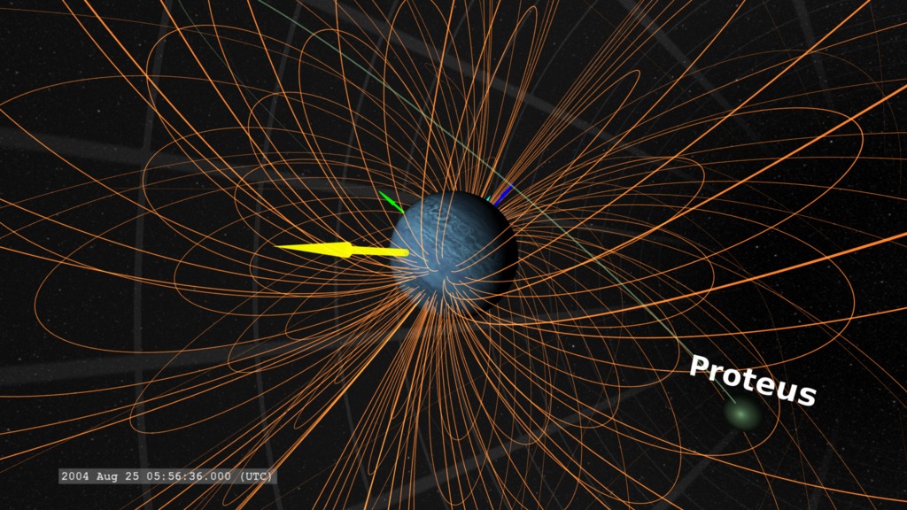
Neptune's Magnetosphere
Go to this pageEarth's magnetic field creates a 'bubble' around Earth that helps protect our planet from some of the more harmful effects of energetic particles streaming out from the sun in the solar wind. Some of the earliest hints of this interaction go back to the 1850s with the work of Richard Carrington, and in the early 1900s with the work of Kristian Birkeland and Carl Stormer. That this field might form a type of 'bubble' around Earth was hypothesized by Sidney Chapman and Vincent Ferraro in the 1930s. The term 'magnetosphere' was applied to magnetic bubble by Thomas Gold in 1959. But it wasn't until the Space Age, when we sent the first probes to other planets, that we found clear evidence of their magnetic fields (though there were hints of a magnetic field for Jupiter in the 1950s, due to observations from radio telescopes). The Voyager program , two spacecraft launched in 1977, and successors to the Pioneer 10 and 11 missions, completed flybys of the giant outer planets. They became the implementation of the 'Grand Tour' of the outer planets originally proposed in the late 1960s. The Voyagers provided some of the first detailed measurments of the strength, extent and diversity of the magnetospheres of the outer planets.In these visualizations, we present simplified models of these planetary magnetospheres, designed to illustrate their scale, and basic features of their structure and impacts of the magnetic axes offset from the planetary rotation axes. The rotation axis of Neptune is highly tilted relative to the revolution axis of the solar system, but nowhere near as extreme as Uranus. It's magnetic axis also has a large tilt relative to the rotation axis. These effects combine to not only give Uranus a more a more variable magnetosphere, but suggest the planet's magnetic field may be generated by a different mechanism than that of Earth, Jupiter and Saturn.For these visualizations, the magnetic field structure is represented by gold/copper lines. Some additional glyphs are provided to indicate some key directions in the field model.The Yellow arrow points towards the sun. The magnetotail is pointed in the opposite direction.The Cyan arrow represents the magnetic axis, usually tilted relative to the rotation axis. The arrow indicates the NORTH magnetic pole (convention has field lines moving north to south as the north pole of bar magnet (and compass pointer) points to the south magnetic pole).The Blue arrow represents the north rotation axis. It is part of the 3-D axis glyph (red, green, and blue arrows) included to make the planetary rotation more apparent.The semi-transparent grey mesh in the distance represents the boundary of the magnetosphere.Major satellites of the planetary system are also included. When appropriate for the time window of the visualization, the Voyager flyby trajectories are indicated.The models are constructed by combining the fields of a simple magnetic dipole, a current sheet (whose intensity is tuned match the scale of the magnetotail), and occasionally a ring current. This is a variation of the simple Luhmann-Friesen magnetosphere model. They are meant to be representative of the basic characteristics of the planetary magnetic fields. Some features NOT included are longitudes of magnetic poles to a standard planetary coordinate system and offsets of the dipole center from the planetary center. ReferencesT. Gold, Motions in the Magnetosphere of the EarthLuhmann & Friesen, A simple model of the magnetosphereMagnetic reconnection at Neptune's magnetopauseLASP: Polarity of planetary magnetic fieldsWikipedia: The Solar Storm of 1859Wikipedia: Kristian BirkelandWikipedia: Carl StørmerSpecial thanks to Arik Posner (NASA/HQ) and Gina DiBraccio (UMBC/GSFC) for helpful pointers on orientation of planetary rotation and magnetic axes. ||
Upper Atmosphere Physics
- ID: 4540 Visualization
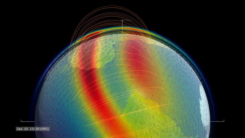
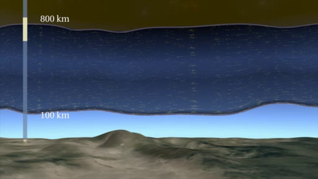
Exploring Earth's Ionosphere: Limb view
Go to this pageThis visualization presents data on the concentration of the singly-ionized oxygen atom (rainbow color table, red is highest concentration), the low-latitude geomagnetic field (gold field lines) and the ionospheric winds at two altitude levels, 100km (white) and 350 km (violet). || IRIDaily.limb_OionHwindIGRF.clockSlate_CRTT.HD1080i.000750_print.jpg (1024x576) [101.4 KB] || IRIDaily.limb_OionHwindIGRF.clockSlate_CRTT.HD1080i.000750_thm.png (80x40) [5.0 KB] || IRIDaily.limb_OionHwindIGRF.clockSlate_CRTT.HD1080i.000750_searchweb.png (320x180) [62.5 KB] || IRIDaily.limb_OionHwindIGRF.HD1080i_p30.mp4 (1920x1080) [88.3 MB] || OionHwindIGRF (1920x1080) [0 Item(s)] || OionHwindIGRF (3840x2160) [0 Item(s)] || IRIDaily.limb_OionHwindIGRF.2160p30.webm (3840x2160) [12.4 MB] || IRIDaily.limb_OionHwindIGRF.2160p30.mp4 (3840x2160) [274.0 MB] || IRIDaily.limb_OionHwindIGRF.HD1080i_p30.mp4.hwshow [205 bytes] ||
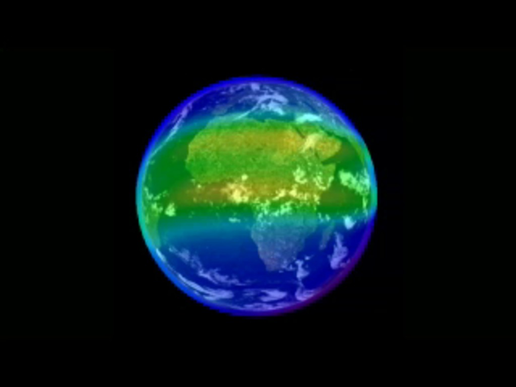
- ID: 4617 Visualization
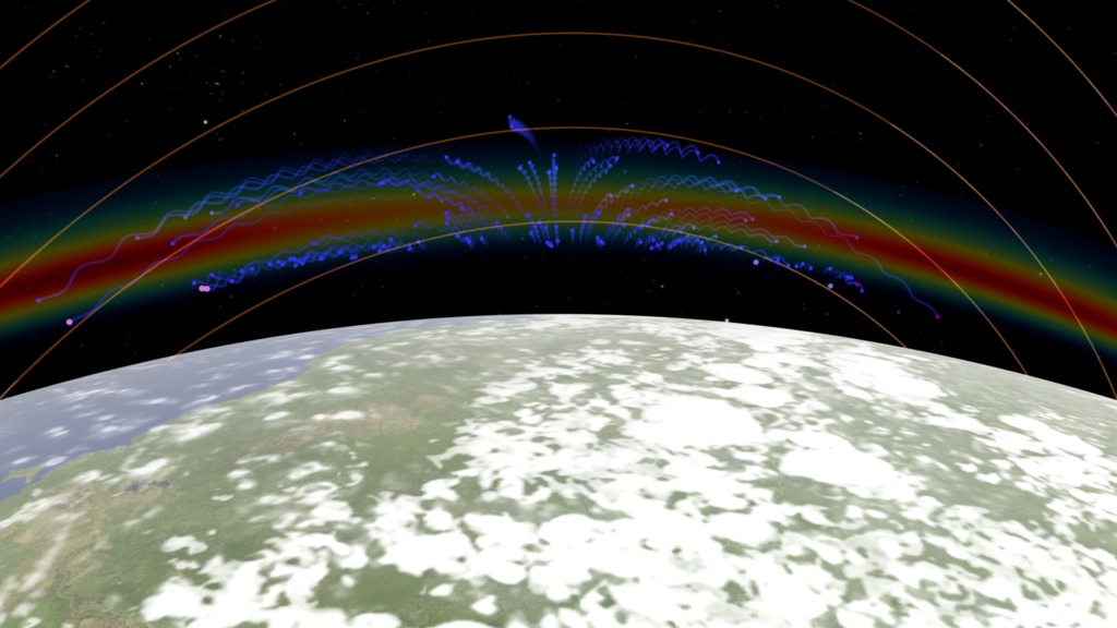
Interface to Space: The Equatorial Fountain
Go to this pageVisualization illustrating the Fountain Effect of ions in the near-Earth electric and magnetic fields. || IRIConceptual.Limb2PullOut_OionFountainIGRF.noslate_CRTT.HD1080i.000660_print.jpg (1024x576) [114.5 KB] || IRIConceptual.Limb2PullOut_OionFountainIGRF.noslate_CRTT.HD1080i.000660_searchweb.png (320x180) [87.8 KB] || IRIConceptual.Limb2PullOut_OionFountainIGRF.noslate_CRTT.HD1080i.000660_thm.png (80x40) [7.2 KB] || 1920x1080_16x9_30p (1920x1080) [0 Item(s)] || IRIConceptual.Limb2PullOut_OionFountainIGRF.HD1080i_p30.mp4 (1920x1080) [32.1 MB] || IRIConceptual.Limb2PullOut_OionFountainIGRF.HD1080i_p30.webm (1920x1080) [4.2 MB] || 3840x2160_16x9_30p (3840x2160) [0 Item(s)] || IRIConceptual.Limb2PullOut_OionFountainIGRF_2160p30.mp4 (3840x2160) [96.1 MB] || IRIConceptual.Limb2PullOut_OionFountainIGRF.HD1080i_p30.mp4.hwshow [221 bytes] ||
- ID: 10342 Produced Video
Ionosphere and CINDI
Go to this pageThe Coupled Ion Dynamics Investigation (CINDI) is a joint NASA/Air Force funded Ionospheric plasma sensor. This animation shows how the ionosphere changes between Daytime and nighttime. ||
- ID: 10208 Produced Video
4D Ionosphere
Go to this pageNASA-funded researchers have unveiled a new '4D' live model of Earth's ionosphere at the Space Weather Workshop, Boulder, CO. Without leaving home, anyone can fly through the dynamic layer of ionized gases that encircles Earth at edge of space itself. All that's required is a connection to the Internet. Airline flight controllers can use this tool to plan long-distance flights over the poles, saving money and time for flyers. ||
- ID: 3484 Visualization
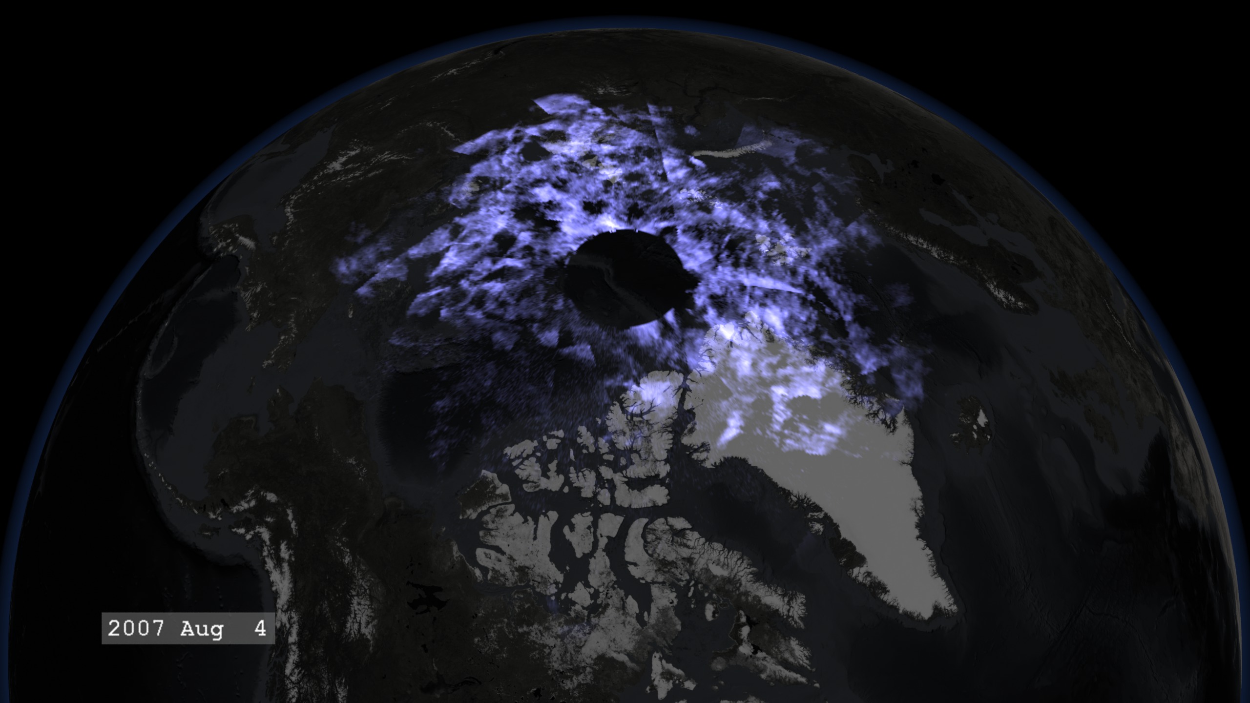
The First Season of Noctilucent Clouds from AIM
Go to this pageThe Aeronomy of Ice in the Mesosphere (AIM) mission is the first satellite dedicated to the study of noctilucent clouds. Noctilucent clouds, sometimes called Polar Mesospheric Clouds, were first reported in 1885. Forming at altitudes above 50 miles, they are so faint that they can only be seen from the ground in the reflected light of the Sun after it has set below the horizon. Since their discovery, their cause has been a subject of study as a possible indicator of climate change. For those interested in observing noctilucent clouds from the ground, there are images and information at SpaceWeather's Gallery of Noctilucent Clouds. ||
Narrated Movies
- ID: 11003 Produced Video
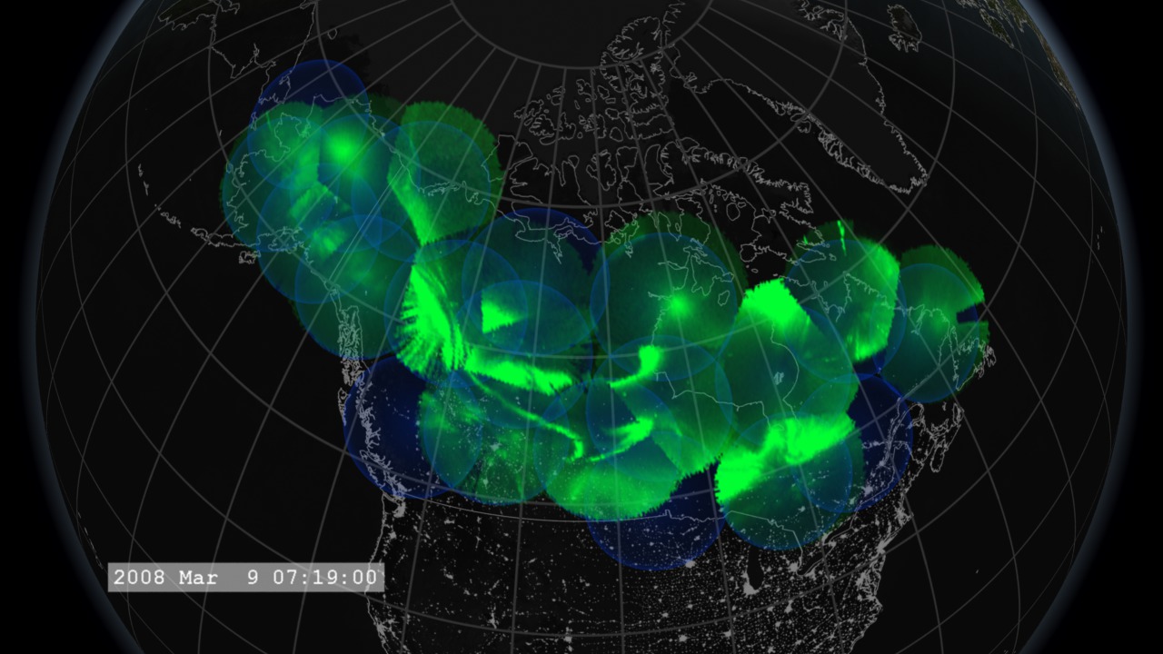
Excerpt from "Dynamic Earth"
Go to this pageA giant explosion of magnetic energy from the sun, called a coronal mass ejection, slams into and is deflected completely by the Earth's powerful magnetic field. The sun also continually sends out streams of light and radiation energy. Earth's atmosphere acts like a radiation shield, blocking quite a bit of this energy.Much of the radiation energy that makes it through is reflected back into space by clouds, ice and snow and the energy that remains helps to drive the Earth system, powering a remarkable planetary engine — the climate. It becomes the energy that feeds swirling wind and ocean currents as cold air and surface waters move toward the equator and warm air and water moves toward the poles — all in an attempt to equalize temperatures around the world.A jury appointed by the National Science Foundation (NSF) and Science magazine has selected "Excerpt from Dynamic Earth" as the winner of the 2013 NSF International Science and Engineering Visualization Challenge for the Video category. This animation will be highlighted in the February 2014 special section of Science and will be hosted on ScienceMag.org and NSF.govThis animation was selected for the Computer Animation Festival's Electronic Theater at the Association for Computer Machinery's Special Interest Group on Computer Graphics and Interactive Techniques (SIGGRAPH), a prestigious computer graphics and technical research forum. This is an excerpt from the fulldome, high-resolution show 'Dynamic Earth: Exploring Earth's Climate Engine.' The Dynamic Earth dome show was selected as a finalist in the Jackson Hole Wildlife Film Festival Science Media Awards under the category "Best Immersive Cinema - Fulldome". ||
- ID: 3595 Visualization
Sentinels of the Heliosphere
Go to this pageHeliophysics is a term to describe the study of the Sun, its atmosphere or the heliosphere, and the planets within it as a system. As a result, it encompasses the study of planetary atmospheres and their magnetic environment, or magnetospheres. These environments are important in the study of space weather.As a society dependent on technology, both in everyday life, and as part of our economic growth, space weather becomes increasingly important. Changes in space weather, either by solar events or geomagnetic events, can disrupt and even damage power grids and satellite communications. Space weather events can also generate x-rays and gamma-rays, as well as particle radiations, that can jeopardize the lives of astronauts living and working in space.This visualization tours the regions of near-Earth orbit; the Earth's magnetosphere, sometimes called geospace; the region between the Earth and the Sun; and finally out beyond Pluto, where Voyager 1 and 2 are exploring the boundary between the Sun and the rest of our Milky Way galaxy. Along the way, we see these regions patrolled by a fleet of satellites that make up NASA's Heliophysics Observatory Telescopes. Many of these spacecraft do not take images in the conventional sense but record fields, particle energies and fluxes in situ. Many of these missions are operated in conjunction with international partners, such as the European Space Agency (ESA) and the Japanese Space Agency (JAXA).The Earth and distances are to scale. Larger objects are used to represent the satellites and other planets for clarity.Here are the spacecraft featured in this movie:Near-Earth Fleet:Hinode: Observes the Sun in multiple wavelengths up to x-rays. SVS pageRHESSI : Observes the Sun in x-rays and gamma-rays. SVS pageTRACE: Observes the Sun in visible and ultraviolet wavelengths. SVS pageTIMED: Studies the upper layers (40-110 miles up) of the Earth's atmosphere.FAST: Measures particles and fields in regions where aurora form.CINDI: Measures interactions of neutral and charged particles in the ionosphere. AIM: Images and measures noctilucent clouds. SVS pageGeospace Fleet:Geotail: Conducts measurements of electrons and ions in the Earth's magnetotail. Cluster: This is a group of four satellites which fly in formation to measure how particles and fields in the magnetosphere vary in space and time. SVS pageTHEMIS: This is a fleet of five satellites to study how magnetospheric instabilities produce substorms. SVS pageL1 Fleet: The L1 point is a Lagrange Point, a point between the Earth and the Sun where the gravitational pull is approximately equal. Spacecraft can orbit this location for continuous coverage of the Sun.SOHO: Studies the Sun with cameras and a multitude of other instruments. SVS pageACE: Measures the composition and characteristics of the solar wind. Wind: Measures particle flows and fields in the solar wind. Heliospheric FleetSTEREO-A and B: These two satellites observe the Sun, with imagers and particle detectors, off the Earth-Sun line, providing a 3-D view of solar activity. SVS pageHeliopause FleetVoyager 1 and 2: These spacecraft conducted the original 'Planetary Grand Tour' of the solar system in the 1970s and 1980s. They have now travelled further than any human-built spacecraft and are still returning measurements of the interplanetary medium. SVS pageThis enhanced, narrated visualization was shown at the SIGGRAPH 2009 Computer Animation Festival in New Orleans, LA in August 2009; an eariler version created for AGU was called NASA's Heliophysics Observatories Study the Sun and Geospace. ||
- ID: 11660 Produced Video
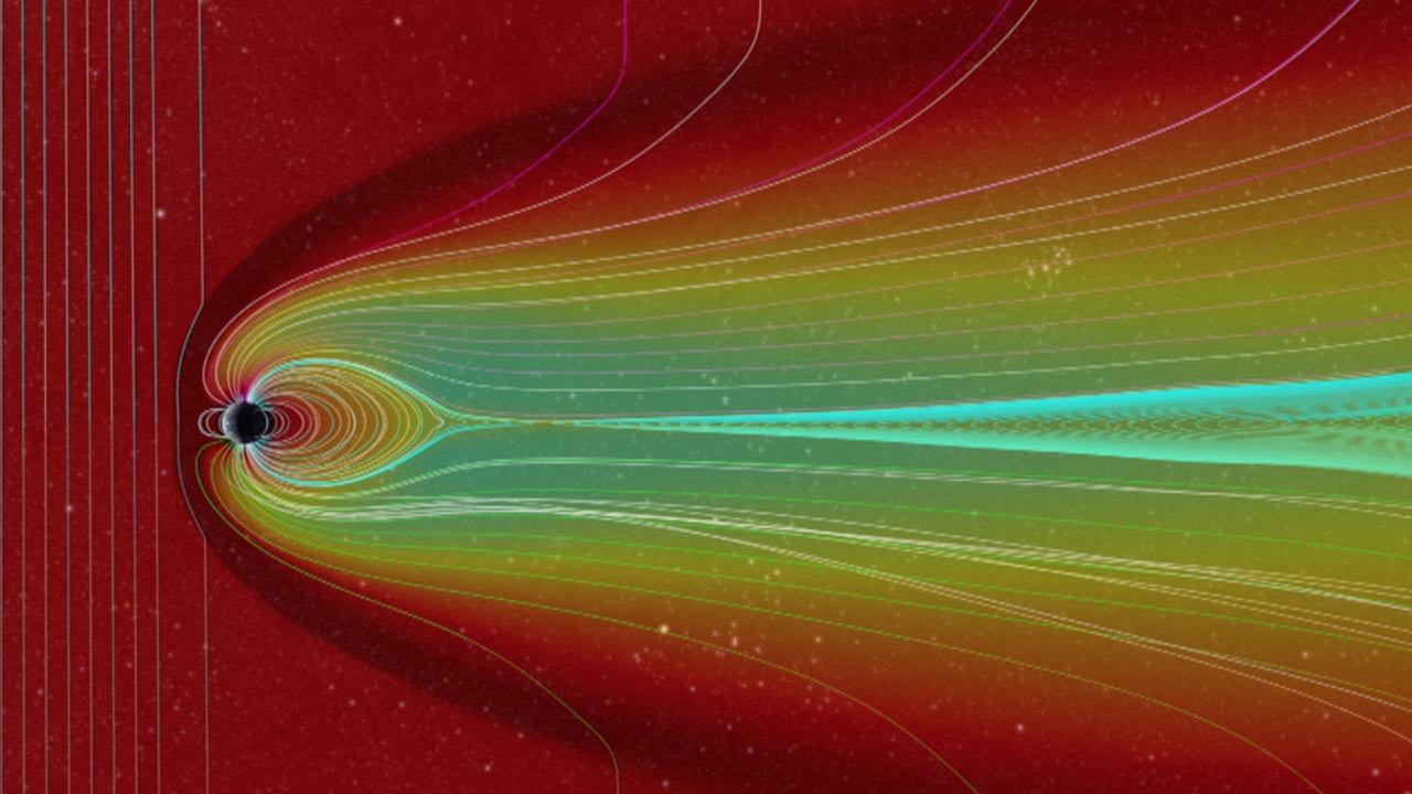
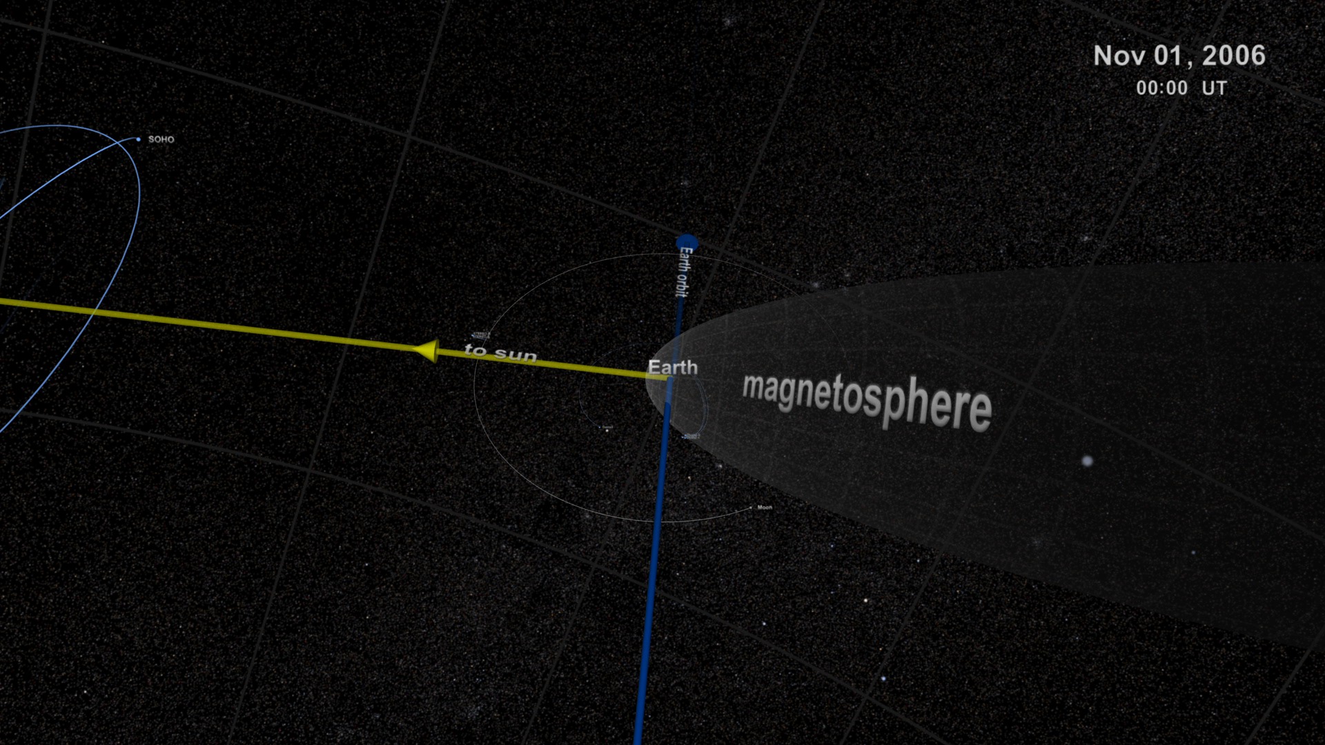
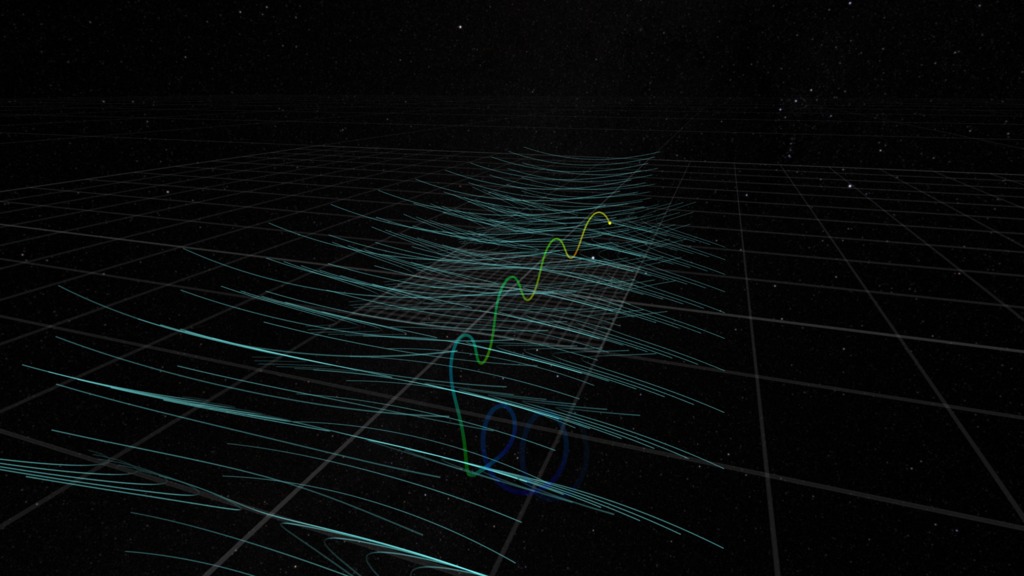
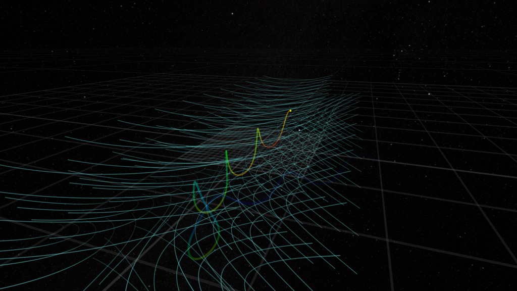
Comparing CMEs
Go to this pageThis video features two model runs. One looks at a moderate coronal mass ejection (CME) from 2006. The second run examines the consequences of a large coronal mass ejection, such as The Carrington-Class CME of 1859. These model runs allow us to estimate consequences of a large event hitting Earth, so we can better protect power grids and satellites.In an effort to understand and predict the impact of space weather events on Earth, the Community-Coordinated Modeling Center (CCMC) at NASA Goddard Space Flight Center, routinely runs computer models of the many historical events. These model runs are then compared to actual data to determine ways to improve the model, and therefore forecasts of future space weather events.Sometimes we need an actual event to have data for comparison. Extreme space weather events are one example where researchers must test models with a rather limited set of data.The vertical lines on the left represent magnetic field lines from the sun. ||
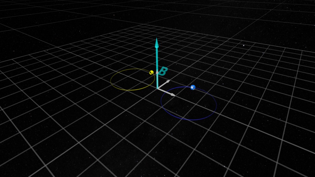
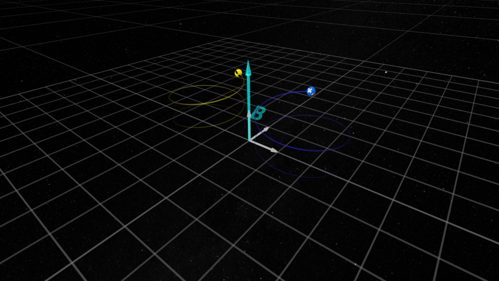
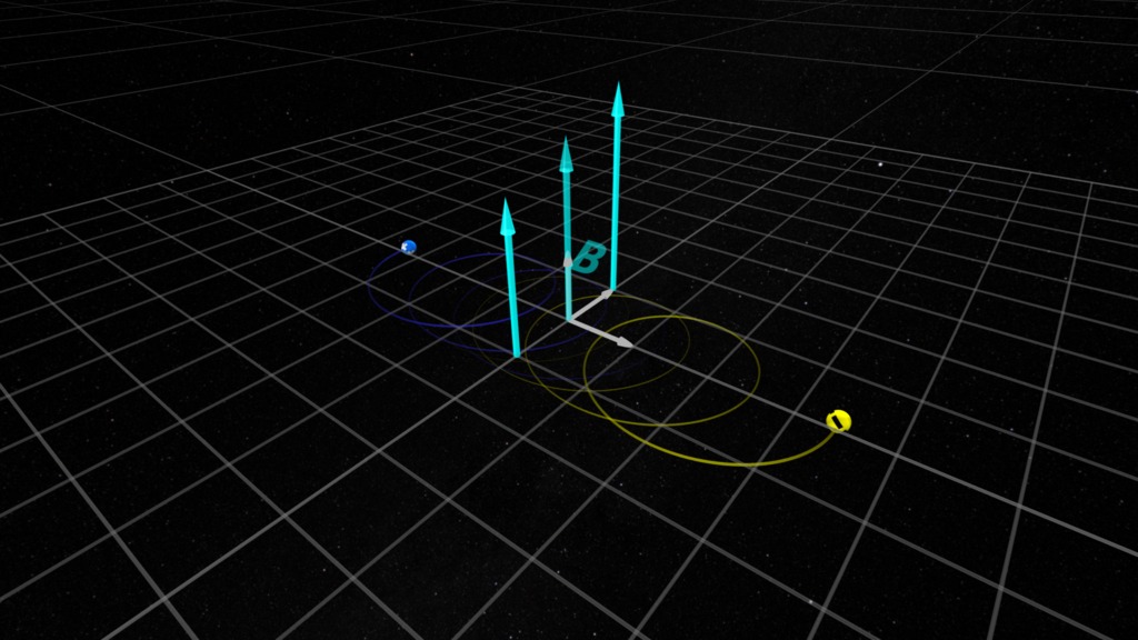
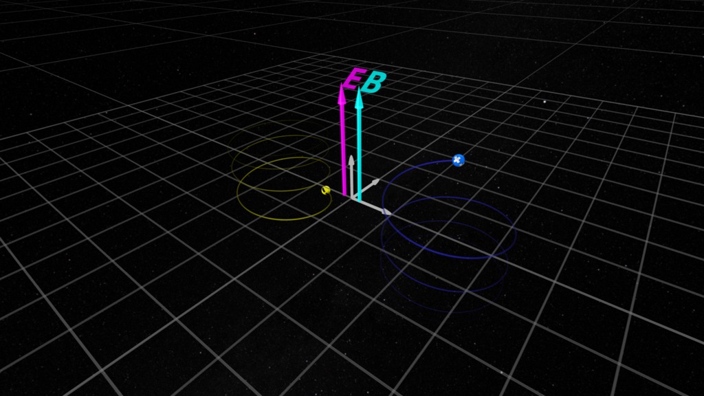
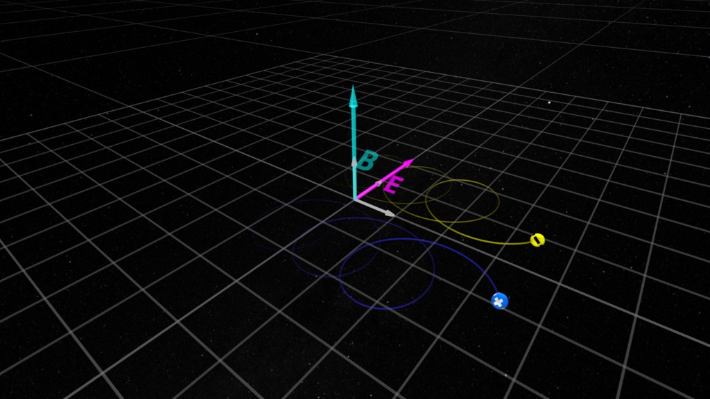
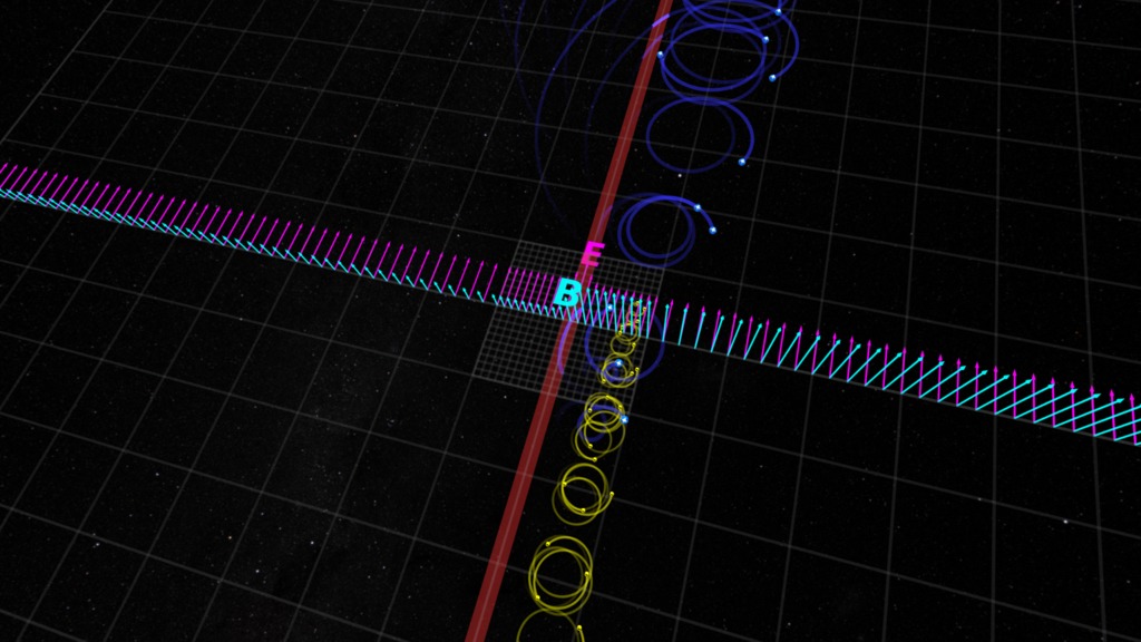
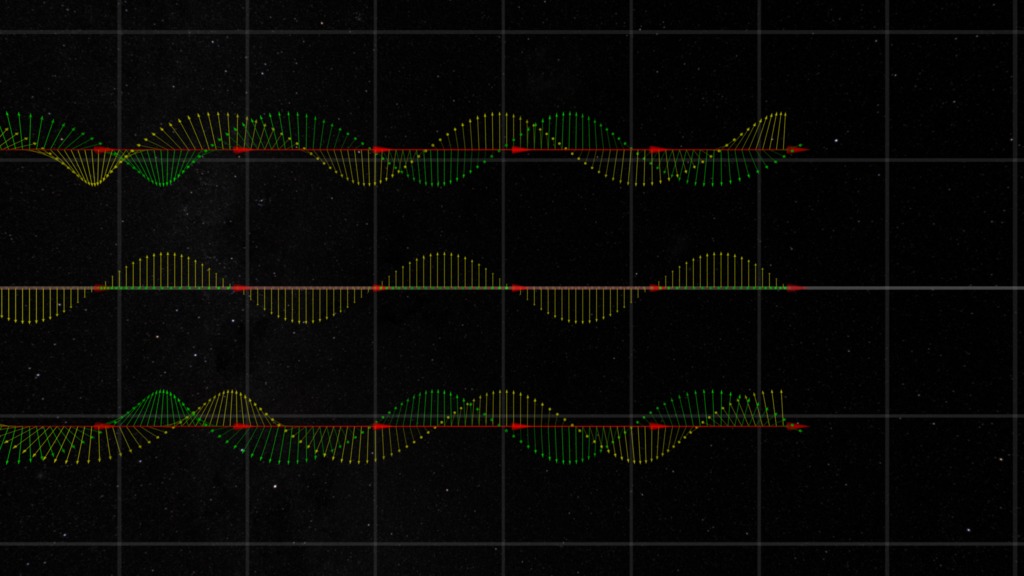
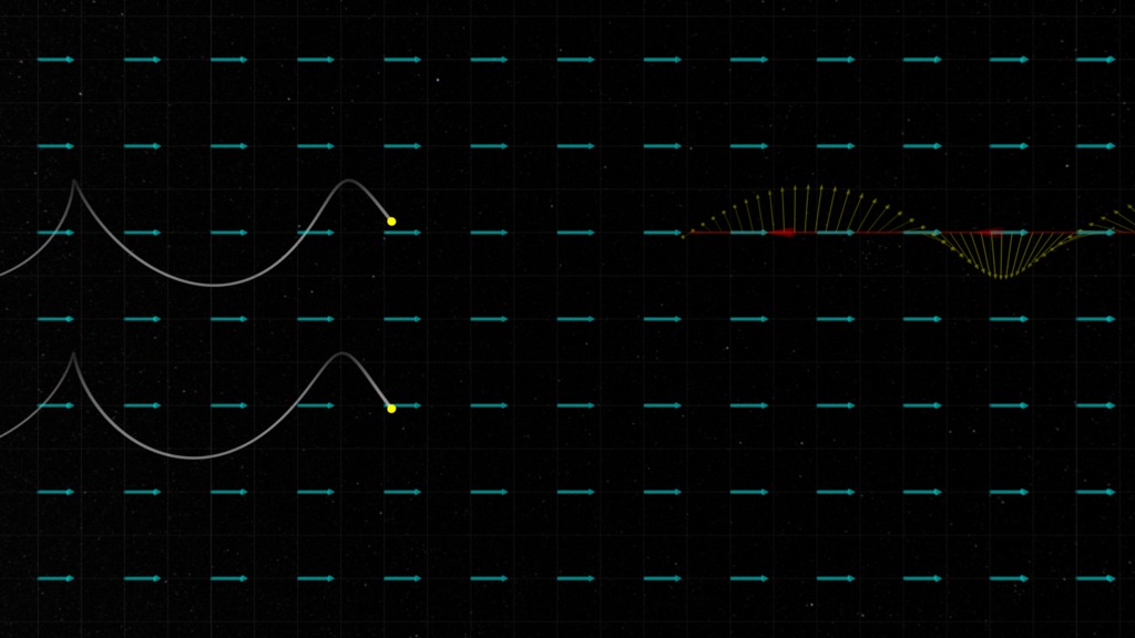
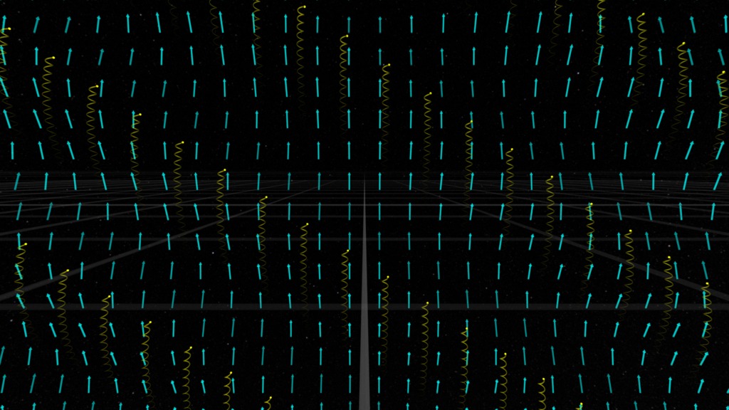
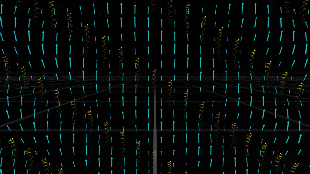
Wave & Plasma Zoo
A collection of visualizations illustrating the different microscopic and macroscopic phenomena observed in electromagnetic waves and plasmas.
- ID: 4261
 Visualization
 - ID: 4262
 Visualization
 - ID: 4263
 Visualization
 - ID: 4264
 Visualization
 - ID: 4265
 Visualization
 - ID: 4513
 Visualization
 - ID: 4580
 Visualization
 - ID: 4649
 Visualization
 - ID: 4560
 Visualization
 - ID: 4561
 Visualization
 - ID: 4568
 Visualization
 - ID: 4569
 Visualization
 - ID: 4987
 Visualization