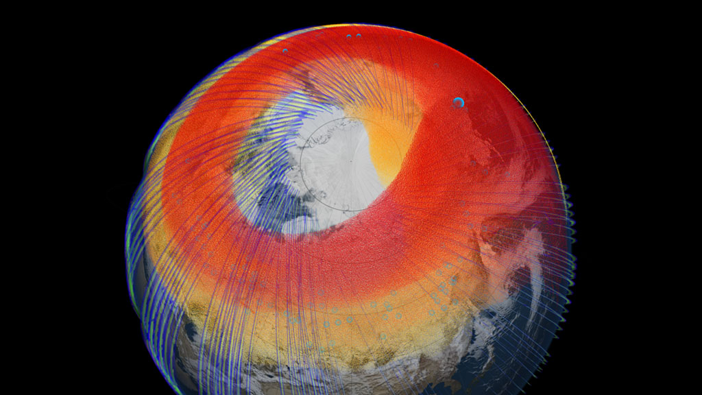
Chelyabinsk Bolide Plume as seen by NPP and NASA Models
Shortly after dawn on Feb. 15, 2013, a bolide measuring 18 meters across and weighing 11,000 metric tons, screamed into Earth's atmosphere at 18.6 kilometers per second. Burning from the friction with Earth's thin air, the space rock exploded 23.3 kilometers above Chelyabinsk, Russia. The event led to the formation of a new dust belt in Earth's stratosphere. Scientists used data from the NASA-NOAA Suomi NPP satellite along with the GEOS-5 computational atmospheric model to achieve the first space-based observation of the long-term evolution of a bolide plume.
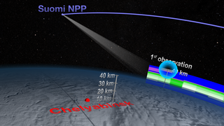
NPP's Ozone Mapping and Profiler Suite (OMPS) Limb instrument first observed the dust plume from the explosion about 1,100 kilometers east of Chelyabinsk, due to the location of the satellite's orbit. NPP's second observation was farther west, close to Chelyabinsk, because the spacecraft's orbit moves from east to west. The third observation of the plume occurred the day following the event. The OMPS instrument could only see the plume during the daytime, and the NPP orbit had progressed westward away from the plume and into night by the time it was again over the plume.
The OMPS Limb instrument observations are made by looking backward (relative to NPP's orbit) toward the Earth's limb. The instrument makes measurements through three separate slits. Early on, some of the plume observations where only made in one or two of the slits, but later observations tended to include all three slits as the plume stretched out.
This visualization shows the how observations by the Suomi NPP satellite's Ozone Mapping and Profiler Suite (OMPS) Limb instrument, and information from the GEOS-5 computational atmospheric model, together revealed the bolide plume snaking around the atmosphere.
For complete transcript, click here.
This video is also available on our YouTube channel.

On Feb. 15, 2013, the bolide was about to explode over Chelyabinsk, Russia.
The Suomi NPP satellite made its first observation 1,100 kilometers from the explosion.
Scientists used the initial satellite measurements of the plume to seed the GEOS-5 computational model.
The location of the satellite's first observation (blue circle) is seen with respect to the modeled plume.
The satellite's second observation is labeled with respect to the modeled plume.
The modeled path and height of the plume continue to agree well with satellite observations.
Four days after the bolide explosion, the faster, higher portion of the plume (red) had snaked its way entirely around the northern hemisphere and back to Chelyabinsk, Russia.
The modeled plume is diffuse, shown here with early Suomi NPP observations.
These vertical profiles of the atmosphere are based on the Suomi NPP satellite's Ozone Mapping and Profiler Suite (OMPS) Limb instrument; measuring at an angle to Earth's surface, the instrument scans tiny slices of the atmosphere through 3 separate slits.
Colors assigned to the GEOS-5 model of the plume which range from 10 km (gray) to 30 km (yellow) to 50 km (red)
Colors assigned to the Suomi NPP data curtains from the OMPS instrument: extinction ranging from 1e-06 (blue) to 1e-05 (purple) to 1e-04 (green) to 1e-03 (white). This is a logarithmic scale.
For More Information
Credits
Please give credit for this item to:
NASA's Goddard Space Flight Center Scientific Visualization Studio
-
Animators
- Greg Shirah (NASA/GSFC)
- Horace Mitchell (NASA/GSFC)
-
Narration
- Silvia Stoyanova (USRA)
-
Narrator
- Mike Velle (HTSI)
-
Producer
- Silvia Stoyanova (USRA)
-
Scientists
- Nick Gorkavyi (SSAI)
- Paul Newman (NASA/GSFC)
- Arlindo M. Da Silva (NASA/GSFC)
Release date
This page was originally published on Wednesday, August 14, 2013.
This page was last updated on Tuesday, November 14, 2023 at 12:04 AM EST.
Series
This visualization can be found in the following series:Datasets used in this visualization
-
CelesTrak Spacecraft Orbit Ephemeris
ID: 454This dataset can be found at: http://celestrak.com
See all pages that use this dataset -
GEOS-5 Cubed-Sphere (GEOS-5 Atmospheric Model on the Cubed-Sphere)
ID: 663The model is the GEOS-5 atmospheric model on the cubed-sphere, run at 14-km global resolution for 30-days. GEOS-5 is described here http://gmao.gsfc.nasa.gov/systems/geos5/ and the cubed-sphere work is described here http://sivo.gsfc.nasa.gov/cubedsphere_overview.html.
See all pages that use this dataset -
Limb Data [Suomi NPP: Ozone Mapping Progiler Suite (OMPS)]
ID: 794
Note: While we identify the data sets used in these visualizations, we do not store any further details, nor the data sets themselves on our site.
Related
- ID: 11325
 Produced Video
 - ID: 11336
 Produced Video